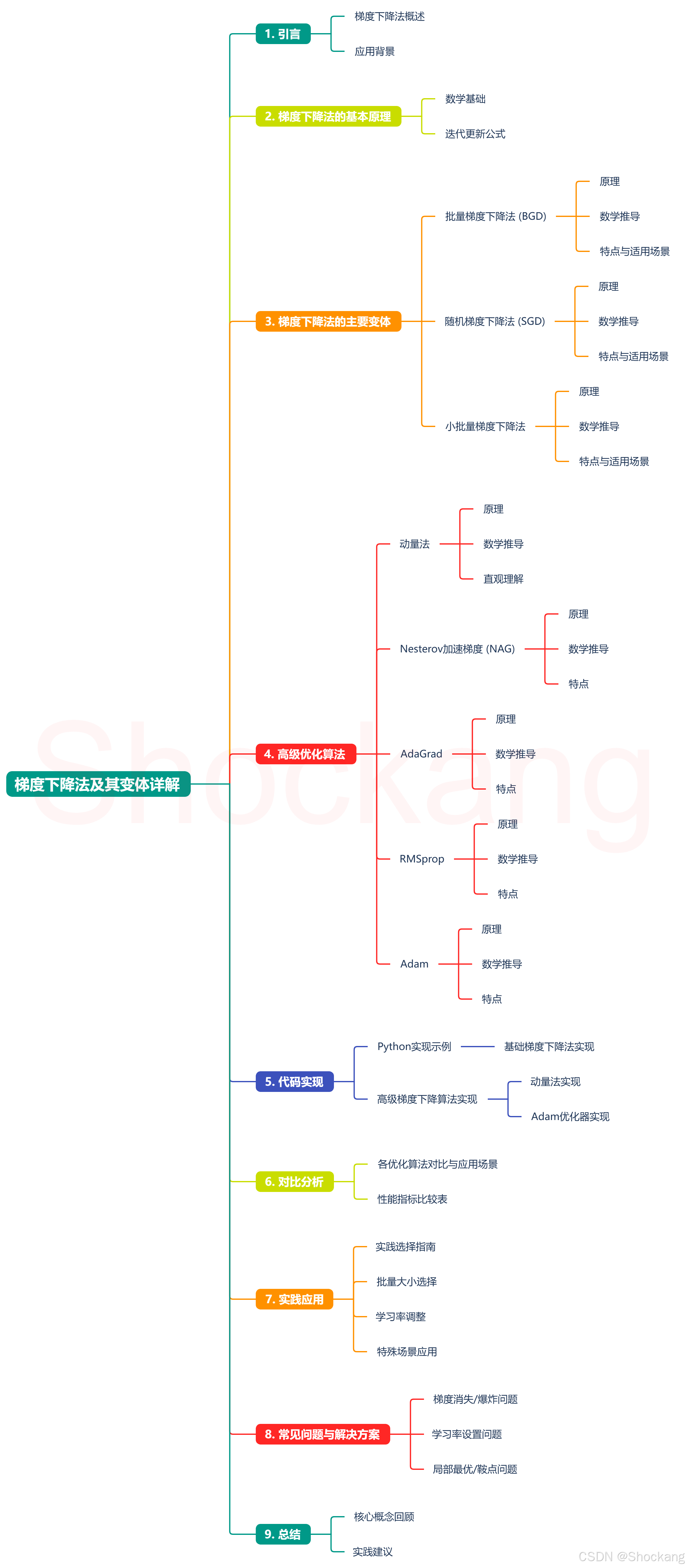
梯度下降法及其变体详解

📚 从数学原理到代码实现，一文掌握梯度下降法全家桶！本文深入浅出地剖析BGD、SGD到Adam等8种优化算法的原理与公式推导，配合Python实例与直观图表，帮你理解参数更新背后的数学逻辑。无论你是算法小白还是寻求进阶，这份"通关指南"都能助你在实战中灵活选择最佳优化器。🚀

Shockang

1295人浏览 · 2025-03-12 21:18:36

Shockang · 2025-03-12 21:18:36 发布

前言

本文隶属于专栏《机器学习数学通关指南》，该专栏为笔者原创，引用请注明来源，不足和错误之处请在评论区帮忙指出，谢谢！

本专栏目录结构和参考文献请见《机器学习数学通关指南》

ima 知识库

知识库广场搜索：

知识库	创建人
机器学习	@Shockang
机器学习数学基础	@Shockang
深度学习	@Shockang

正文

在这里插入图片描述

📝 引言

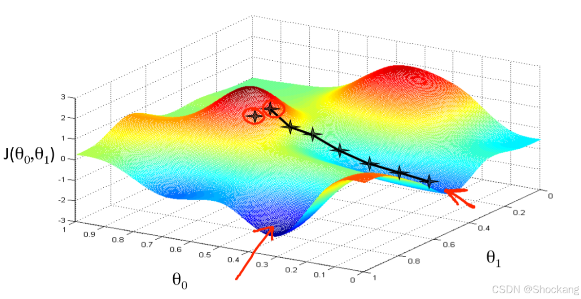
梯度下降法是机器学习和深度学习中最核心的优化算法之一，它通过迭代调整模型参数以最小化损失函数。本文将深入浅出地讲解梯度下降法及其变体的原理、数学推导和应用场景，帮助你在实践中灵活选择最适合的优化方法。

🔍 梯度下降法的基本原理

🧮 数学基础

梯度下降法的核心思想是沿着损失函数的负梯度方向调整参数，以逐步接近损失函数的最小值。

梯度向量 $\nabla J(\theta)$ 指向函数值增长最快的方向，因此沿着负梯度方向 $-\nabla J(\theta)$ 移动可以最快地减小函数值。

在这里插入图片描述

🔄 迭代更新公式

基本的参数更新公式为：

$\theta_{t+1} = \theta_t - \eta \nabla J(\theta_t)$

其中：

$\theta$ 是模型参数
$\eta$ 是学习率（步长）
$\nabla J(\theta)$ 是损失函数的梯度

🚶‍♂️ 梯度下降法的主要变体

1️⃣ 批量梯度下降法 (Batch Gradient Descent, BGD)

原理

每次迭代使用全部训练数据计算梯度并更新参数。

数学推导

损失函数为全体数据的平均损失：
$J(\theta) = \frac{1}{N} \sum_{i=1}^N J_i(\theta)$

参数更新公式：
$\theta_{t+1} = \theta_t - \eta \cdot \frac{1}{N} \sum_{i=1}^N \nabla J_i(\theta_t)$

特点

✅ 优点：梯度估计准确，收敛稳定，对于凸函数可收敛至全局最优
❌ 缺点：计算成本高，内存消耗大，不适合大规模数据集
🎯 适用场景：小规模数据集，需要精确解的问题

2️⃣ 随机梯度下降法 (Stochastic Gradient Descent, SGD)

原理

每次迭代随机选择一个样本计算梯度并更新参数。

数学推导

在随机选取的样本 $x_i, y_i)$ 上更新参数：
$\theta_{t+1} = \theta_t - \eta \cdot \nabla J_i(\theta_t)$

特点

✅ 优点：计算速度快，适合在线学习，能够跳出局部最优
❌ 缺点：更新方向波动大，收敛路径不稳定，需要逐步降低学习率
🎯 适用场景：大规模数据集，在线学习任务

3️⃣ 小批量梯度下降法 (Mini-batch Gradient Descent)

原理

每次迭代使用小批量样本（通常为32、64、128等）计算梯度，是批量梯度下降与随机梯度下降的折中方案。

数学推导

设选取的批量大小为 $B$ ，参数更新公式：
$\theta_{t+1} = \theta_t - \eta \cdot \frac{1}{B} \sum_{i=1}^B \nabla J_i(\theta_t)$

特点

✅ 优点：兼顾计算效率和更新稳定性，可充分利用矩阵运算加速
❌ 缺点：需要调整批量大小这一超参数
🎯 适用场景：现代深度学习中的标准选择，适合大多数问题

🚀 高级优化算法

4️⃣ 动量法 (Momentum)

原理

引入动量项，模拟物理系统中的惯性，累积历史梯度信息，加速收敛并减少震荡。

数学推导

动量初始化为 $v_0 = 0$ ，随后更新过程为：
$v_t = \gamma v_{t-1} + \eta \nabla J(\theta_t)$
$\theta_{t+1} = \theta_t - v_t$

其中 $\gamma$ 是动量系数（通常为0.9），表示历史梯度的衰减率。

直观理解

将梯度累积到动量向量中
梯度方向一致时，加速参数更新
梯度方向震荡时，减少摆动

动量法示意图

5️⃣ Nesterov加速梯度 (NAG)

原理

动量法的改进版，先沿动量方向移动，再计算梯度并调整。

数学推导

$v_t = \gamma v_{t-1} + \eta \nabla J(\theta_t - \gamma v_{t-1})$
$\theta_{t+1} = \theta_t - v_t$

特点

✅ 优点：比标准动量法有更好的收敛性能
🎯 适用场景：需要更快收敛速度的优化问题

6️⃣ AdaGrad

原理

自适应调整每个参数的学习率，为频繁更新的参数使用较小的学习率，为不常更新的参数使用较大的学习率。

数学推导

累积平方梯度：
$G_t = G_{t-1} + (\nabla J(\theta_t))^2$

参数更新：
$\theta_{t+1} = \theta_t - \frac{\eta}{\sqrt{G_t + \epsilon}} \odot \nabla J(\theta_t)$

其中 $\epsilon$ 是小常数（如1e-8），防止除零； $\odot$ 表示元素级乘法。

特点

✅ 优点：适合处理稀疏特征
❌ 缺点：学习率会单调递减，可能过早停止学习
🎯 适用场景：自然语言处理等稀疏特征场景

7️⃣ RMSprop

原理

AdaGrad的改进版，使用指数加权移动平均而非简单累加处理历史梯度。

数学推导

$G_t = \beta G_{t-1} + (1-\beta)(\nabla J(\theta_t))^2$
$\theta_{t+1} = \theta_t - \frac{\eta}{\sqrt{G_t + \epsilon}} \odot \nabla J(\theta_t)$

其中 $\beta$ 通常取0.9。

特点

✅ 优点：解决了AdaGrad学习率过早下降的问题
🎯 适用场景：非凸优化问题，如深度神经网络

8️⃣ Adam (Adaptive Moment Estimation)

原理

结合动量法和RMSprop的优点，同时维护一阶矩（动量）和二阶矩（梯度平方的指数移动平均）。

数学推导

计算一阶矩和二阶矩：
$m_t = \beta_1 m_{t-1} + (1-\beta_1) \nabla J(\theta_t)$
$v_t = \beta_2 v_{t-1} + (1-\beta_2) (\nabla J(\theta_t))^2$

偏差校正：
$\hat{m}_t = \frac{m_t}{1-\beta_1^t}, \quad \hat{v}_t = \frac{v_t}{1-\beta_2^t}$

参数更新：
$\theta_{t+1} = \theta_t - \eta \frac{\hat{m}_t}{\sqrt{\hat{v}_t} + \epsilon}$

通常 $\beta_1=0.9, \beta_2=0.999, \epsilon=10^{-8}$

特点

✅ 优点：综合了动量和自适应学习率的优势，收敛快，表现稳定
🎯 适用场景：复杂模型训练，尤其是深度学习领域的标准选择

💻 Python实现示例

让我们通过一个简单的线性回归例子来实践不同的梯度下降算法：

import numpy as np
import matplotlib.pyplot as plt

# 生成示例数据
np.random.seed(42)
X = 2 * np.random.rand(100, 1)
y = 4 + 3 * X + np.random.randn(100, 1)

# 批量梯度下降
def batch_gradient_descent(X, y, learning_rate=0.1, n_iterations=1000):
    m = len(y)
    X_b = np.c_[np.ones((m, 1)), X]  # 添加偏置项
    theta = np.random.randn(2, 1)    # 随机初始化参数
    
    cost_history = []
    theta_history = []
    
    for iteration in range(n_iterations):
        gradients = 2/m * X_b.T.dot(X_b.dot(theta) - y)
        theta = theta - learning_rate * gradients
        theta_history.append(theta.copy())
        
        cost = np.mean((X_b.dot(theta) - y) ** 2)
        cost_history.append(cost)
    
    return theta, cost_history, theta_history

# 随机梯度下降
def stochastic_gradient_descent(X, y, learning_rate=0.01, n_iterations=50):
    m = len(y)
    X_b = np.c_[np.ones((m, 1)), X]  # 添加偏置项
    theta = np.random.randn(2, 1)    # 随机初始化参数
    
    cost_history = []
    theta_history = []
    
    for iteration in range(n_iterations):
        for i in range(m):
            random_index = np.random.randint(m)
            xi = X_b[random_index:random_index+1]
            yi = y[random_index:random_index+1]
            gradients = 2 * xi.T.dot(xi.dot(theta) - yi)
            theta = theta - learning_rate * gradients
            theta_history.append(theta.copy())
            
            cost = np.mean((X_b.dot(theta) - y) ** 2)
            cost_history.append(cost)
    
    return theta, cost_history, theta_history

# 小批量梯度下降
def mini_batch_gradient_descent(X, y, learning_rate=0.01, n_iterations=50, batch_size=20):
    m = len(y)
    X_b = np.c_[np.ones((m, 1)), X]  # 添加偏置项
    theta = np.random.randn(2, 1)    # 随机初始化参数
    
    n_batches = int(np.ceil(m / batch_size))
    cost_history = []
    theta_history = []
    
    for iteration in range(n_iterations):
        shuffled_indices = np.random.permutation(m)
        X_b_shuffled = X_b[shuffled_indices]
        y_shuffled = y[shuffled_indices]
        
        for batch_index in range(n_batches):
            start_idx = batch_index * batch_size
            end_idx = min((batch_index + 1) * batch_size, m)
            
            Xi = X_b_shuffled[start_idx:end_idx]
            yi = y_shuffled[start_idx:end_idx]
            
            gradients = 2/len(Xi) * Xi.T.dot(Xi.dot(theta) - yi)
            theta = theta - learning_rate * gradients
            theta_history.append(theta.copy())
            
            cost = np.mean((X_b.dot(theta) - y) ** 2)
            cost_history.append(cost)
    
    return theta, cost_history, theta_history

# 使用不同的梯度下降方法训练模型
theta_bgd, cost_history_bgd, _ = batch_gradient_descent(X, y)
theta_sgd, cost_history_sgd, _ = stochastic_gradient_descent(X, y)
theta_mbgd, cost_history_mbgd, _ = mini_batch_gradient_descent(X, y)

# 打印结果
print("Batch Gradient Descent:", theta_bgd.T)
print("Stochastic Gradient Descent:", theta_sgd.T)
print("Mini-batch Gradient Descent:", theta_mbgd.T)

# 绘制学习曲线
plt.figure(figsize=(10, 6))
plt.plot(cost_history_bgd, label='Batch GD')
plt.plot(np.arange(len(cost_history_sgd))/len(cost_history_sgd)*len(cost_history_bgd), 
         cost_history_sgd, label='SGD')
plt.plot(np.arange(len(cost_history_mbgd))/len(cost_history_mbgd)*len(cost_history_bgd), 
         cost_history_mbgd, label='Mini-batch GD')
plt.xlabel('Iterations')
plt.ylabel('Cost')
plt.legend()
plt.title('Learning curves for different optimizers')
plt.show()

🧩 高级梯度下降算法实现

# 动量法
def momentum_optimizer(X, y, learning_rate=0.01, momentum=0.9, n_iterations=1000):
    m = len(y)
    X_b = np.c_[np.ones((m, 1)), X]  # 添加偏置项
    theta = np.random.randn(2, 1)    # 随机初始化参数
    velocity = np.zeros_like(theta)  # 初始化速度为0
    
    cost_history = []
    
    for iteration in range(n_iterations):
        gradients = 2/m * X_b.T.dot(X_b.dot(theta) - y)
        velocity = momentum * velocity - learning_rate * gradients
        theta = theta + velocity
        
        cost = np.mean((X_b.dot(theta) - y) ** 2)
        cost_history.append(cost)
    
    return theta, cost_history

# Adam优化器
def adam_optimizer(X, y, learning_rate=0.01, beta1=0.9, beta2=0.999, 
                   epsilon=1e-8, n_iterations=1000):
    m = len(y)
    X_b = np.c_[np.ones((m, 1)), X]  # 添加偏置项
    theta = np.random.randn(2, 1)    # 随机初始化参数
    
    # 初始化动量和二阶矩
    m_t = np.zeros_like(theta)
    v_t = np.zeros_like(theta)
    
    cost_history = []
    
    for t in range(1, n_iterations + 1):
        gradients = 2/m * X_b.T.dot(X_b.dot(theta) - y)
        
        # 更新动量和二阶矩估计
        m_t = beta1 * m_t + (1 - beta1) * gradients
        v_t = beta2 * v_t + (1 - beta2) * gradients**2
        
        # 偏差校正
        m_t_corrected = m_t / (1 - beta1**t)
        v_t_corrected = v_t / (1 - beta2**t)
        
        # 更新参数
        theta = theta - learning_rate * m_t_corrected / (np.sqrt(v_t_corrected) + epsilon)
        
        cost = np.mean((X_b.dot(theta) - y) ** 2)
        cost_history.append(cost)
    
    return theta, cost_history

📊 各优化算法对比与应用场景

算法	计算量	内存需求	收敛稳定性	适用场景	超参数难度
批量梯度下降	🔴 高	🔴 高	🟢 高	小规模数据，凸优化问题	🟢 低
随机梯度下降	🟢 低	🟢 低	🔴 低	大规模数据，在线学习	🟡 中
小批量梯度下降	🟡 中	🟡 中	🟡 中	大多数深度学习任务	🟡 中
动量法	🟡 中	🟡 中	🟢 高	高曲率问题，局部最优	🟡 中
NAG	🟡 中	🟡 中	🟢 高	需要更快收敛的问题	🟡 中
AdaGrad	🟡 中	🟡 中	🟡 中	稀疏特征问题	🟡 中
RMSprop	🟡 中	🟡 中	🟡 中	非凸优化问题	🟡 中
Adam	🟡 中	🔴 高	🟢 高	大多数深度学习任务	🔴 高

🔧 实践选择指南

在实际应用中，如何选择合适的优化算法？以下是一些实用建议：

初始尝试：先使用 Adam 优化器，它在大多数情况下表现良好
批量大小选择：
- 大批量（如512-1024）：更准确的梯度估计，更好的并行性
- 小批量（如32-64）：更好的正则化效果，更容易逃离局部最优
学习率调整：
- 常用范围：0.1、0.01、0.001、0.0001
- 学习率衰减：指数衰减、步进衰减、余弦退火等
特殊场景：
- 稀疏数据：可考虑 AdaGrad/Adam
- 序列模型：RMSprop/Adam 通常表现更好
- 计算资源受限：SGD+Momentum 可能是更好的选择