【2025版】怎么构建一个机器学习模型,从零基础到精通,精通收藏这篇就够了!
大家好!今天我将带领大家一步步的来构建一个机器学习模型。我们将按照以下步骤开发客户流失预测分类模型。业务理解数据收集和准备建立机器学习模型模型优化模型部署在开发任何机器学习模型之前,我们必须了解为什么要开发该模型。这里,我们以客户流失预测为例。在这种情况下,企业需要避免公司进一步流失,并希望对流失概率高的客户采取行动。有了上述业务需求,所以需要开发一个客户流失预测模型。数据是任何机器学习项
大家好!
今天我将带领大家一步步的来构建一个机器学习模型。
我们将按照以下步骤开发客户流失预测分类模型。
-
业务理解
-
数据收集和准备
-
建立机器学习模型
-
模型优化
-
模型部署
1.业务理解
在开发任何机器学习模型之前,我们必须了解为什么要开发该模型。
这里,我们以客户流失预测为例。
在这种情况下,企业需要避免公司进一步流失,并希望对流失概率高的客户采取行动。有了上述业务需求,所以需要开发一个客户流失预测模型。
2.数据收集和准备
数据采集
数据是任何机器学习项目的核心。没有数据,我们就无法训练机器学习模型。
在现实情况下,干净的数据并不容易获得。通常,我们需要通过应用程序、调查和许多其他来源收集数据,然后将其存储在数据存储中。
在我们的案例中,我们将使用来自 Kaggle 的电信客户流失数据。它是有关电信行业客户历史的开源分类数据,带有流失标签。
https://www.kaggle.com/datasets/blastchar/telco-customer-churn
探索性数据分析 (EDA) 和数据清理
首先,我们加载数据集。
import pandas as pd

df = pd.read_csv('WA_Fn-UseC_-Telco-Customer-Churn.csv')
df.head()
接下来,我们将探索数据以了解我们的数据集。
以下是我们将为 EDA 流程执行的一些操作。
-
检查特征和汇总统计数据。
-
检查特征中是否存在缺失值。
-
分析标签的分布(流失)。
-
为数值特征绘制直方图,为分类特征绘制条形图。
-
为数值特征绘制相关热图。
-
使用箱线图识别分布和潜在异常值。
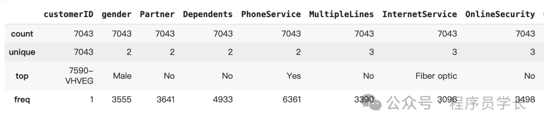
首先,我们将检查特征和汇总统计数据。
df.info()
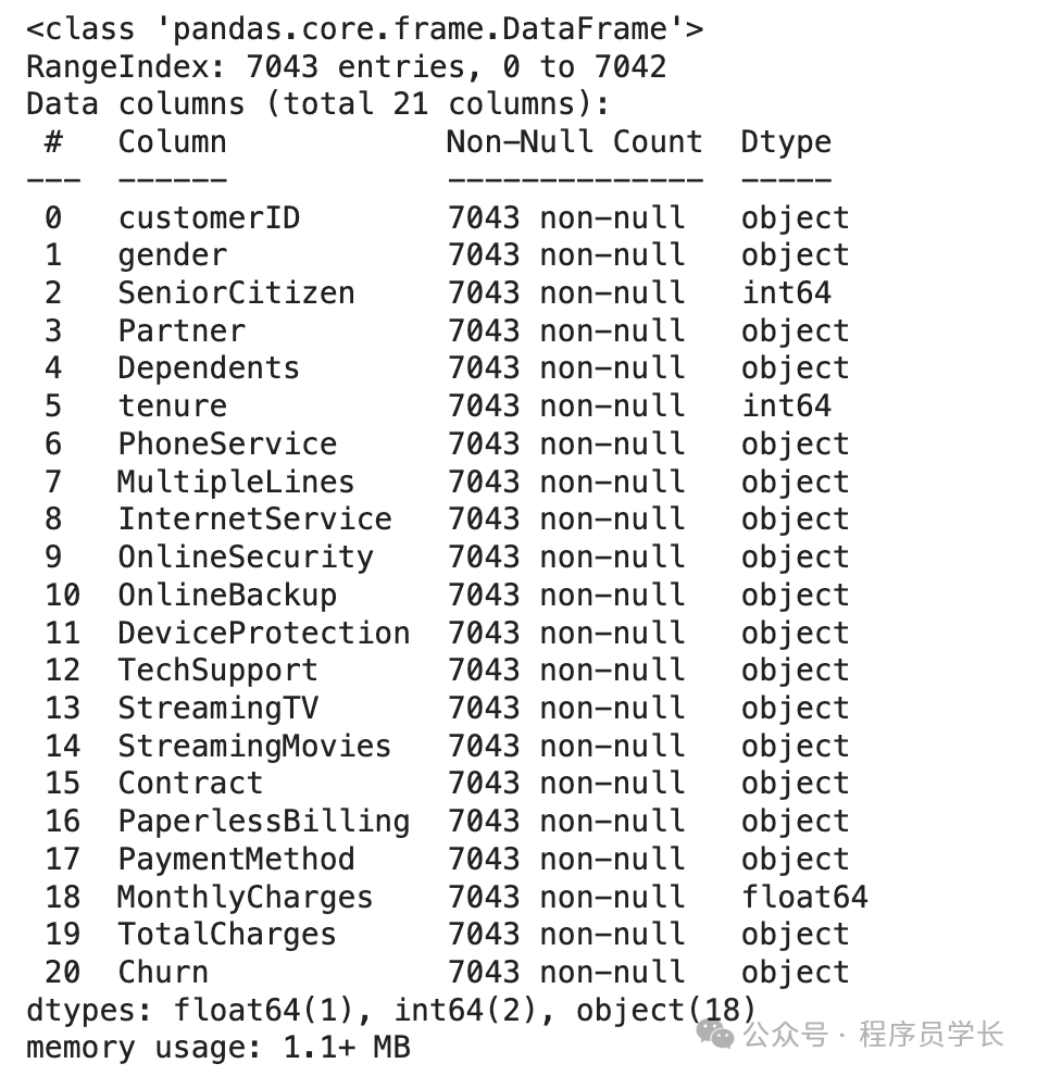
df.describe()

df.describe(exclude = 'number')
让我们检查一下缺失的数据。
df.isnull().sum()
可以看到,数据集不包含缺失数据,因此我们不需要执行任何缺失数据处理活动。
然后,我们将检查目标变量以查看是否存在不平衡情况。
df['Churn'].value_counts()

存在轻微的不平衡,因为与无客户流失的情况相比,只有接近 25% 的客户流失发生。
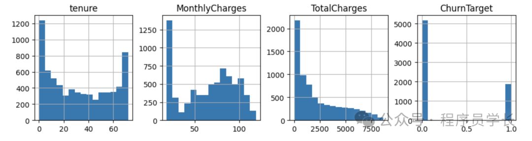
让我们再看看其他特征的分布情况,从数字特征开始。
import numpy as np
df\['TotalCharges'\] = df\['TotalCharges'\].replace('', np.nan)
df\['TotalCharges'\] = pd.to\_numeric(df\['TotalCharges'\], errors='coerce').fillna(0)

df\['SeniorCitizen'\] = df\['SeniorCitizen'\].astype('str')

df\['ChurnTarget'\] = df\['Churn'\].apply(lambda x: 1 if x=='Yes' else 0)

num\_features = df.select\_dtypes('number').columns
df\[num\_features\].hist(bins=15, figsize=(15, 6), layout=(2, 5))
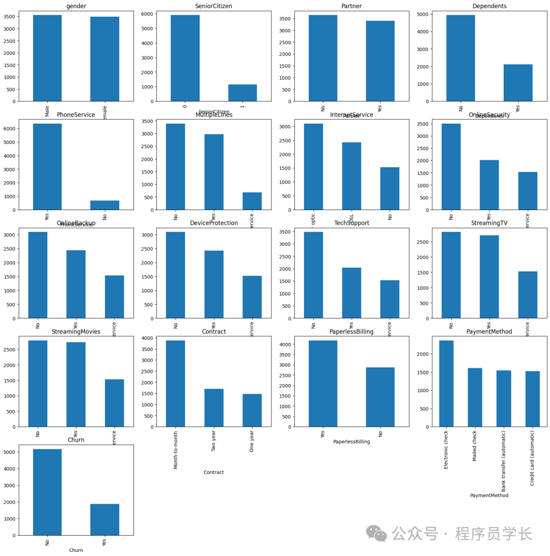
我们还将提供除 customerID 之外的分类特征绘图。
import matplotlib.pyplot as plt
# Plot distribution of categorical features
cat\_features = df.drop('customerID', axis =1).select\_dtypes(include='object').columns

plt.figure(figsize=(20, 20))
for i, col in enumerate(cat\_features, 1):
    plt.subplot(5, 4, i)
    df\[col\].value\_counts().plot(kind='bar')
    plt.title(col)
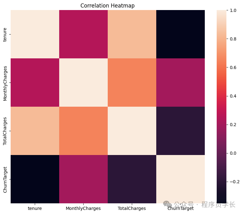
然后我们将通过以下代码看到数值特征之间的相关性。
import seaborn as sns

# Plot correlations between numerical features
plt.figure(figsize=(10, 8))
sns.heatmap(df[num_features].corr())
plt.title('Correlation Heatmap')
最后,我们将使用基于四分位距(IQR)的箱线图检查数值异常值。
# Plot box plots to identify outliers
plt.figure(figsize=(20, 15))
for i, col in enumerate(num_features, 1):
    plt.subplot(4, 4, i)
    sns.boxplot(y=df[col])
    plt.title(col)
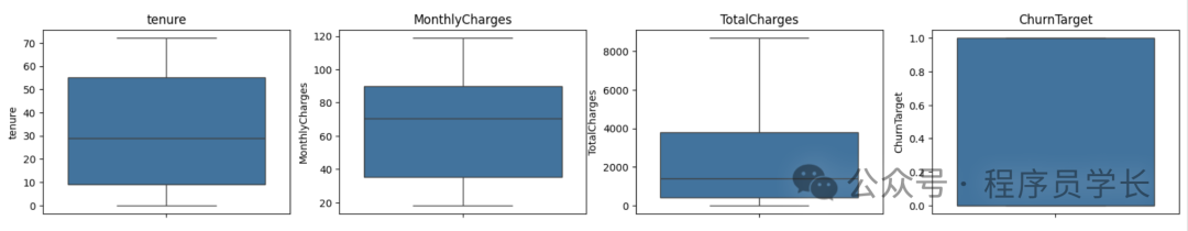
从上面的分析中,我们可以看出,我们不应该解决缺失数据或异常值的问题。
下一步是对我们的机器学习模型进行特征选择,因为我们只想要那些影响预测且在业务中可行的特征。
特征选择
特征选择的方法有很多种,通常结合业务知识和技术应用来完成。
但是,本教程将仅使用我们之前做过的相关性分析来进行特征选择。
首先,让我们根据相关性分析选择数值特征。
target = 'ChurnTarget'
num_features = df.select_dtypes(include=[np.number]).columns.drop(target)

# Calculate correlations
correlations = df[num_features].corrwith(df[target])

# Set a threshold for feature selection
threshold = 0.3
selected_num_features = correlations[abs(correlations) > threshold].index.tolist()
selected_cat_features=cat_features[:-1]

selected_features = []
selected_features.extend(selected_num_features)
selected_features.extend(selected_cat_features)
selected_features
你可以稍后尝试调整阈值,看看特征选择是否会影响模型的性能。
3.建立机器学习模型
选择正确的模型
选择合适的机器学习模型需要考虑很多因素,但始终取决于业务需求。
以下几点需要记住:
-
用例问题。它是监督式的还是无监督式的?是分类式的还是回归式的?用例问题将决定可以使用哪种模型。
-
数据特征。它是表格数据、文本还是图像?数据集大小是大还是小?根据数据集的不同,我们选择的模型可能会有所不同。
-
模型的解释难度如何?平衡可解释性和性能对于业务至关重要。
经验法则是,在开始复杂模型之前,最好先以较简单的模型作为基准。
对于本教程,我们从逻辑回归开始进行模型开发。
分割数据
下一步是将数据拆分为训练、测试和验证集。
from sklearn.model_selection import train_test_split

target = 'ChurnTarget'

X = df[selected_features]
y = df[target]

cat_features = X.select_dtypes(include=['object']).columns.tolist()
num_features = X.select_dtypes(include=['number']).columns.tolist()

#Splitting data into Train, Validation, and Test Set
X_train_val, X_test, y_train_val, y_test = train_test_split(X, y, test_size=0.2, random_state=42, stratify=y)

X_train, X_val, y_train, y_val = train_test_split(X_train_val, y_train_val, test_size=0.25, random_state=42, stratify=y_train_val)
在上面的代码中,我们将数据分成 60% 的训练数据集和 20% 的测试和验证集。
一旦我们有了数据集,我们就可以训练模型。
训练模型
如上所述,我们将使用训练数据训练 Logistic 回归模型。
from sklearn.compose import ColumnTransformer
from sklearn.pipeline import Pipeline
from sklearn.preprocessing import OneHotEncoder
from sklearn.linear_model import LogisticRegression


preprocessor = ColumnTransformer(
    transformers=[
        ('num', 'passthrough', num_features),
        ('cat', OneHotEncoder(), cat_features)
    ])

pipeline = Pipeline(steps=[
    ('preprocessor', preprocessor),
    ('classifier', LogisticRegression(max_iter=1000))
])

# Train the logistic regression model
pipeline.fit(X_train, y_train)
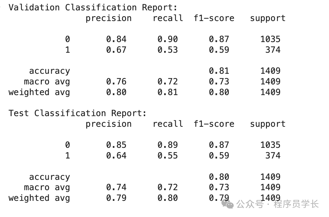
模型评估
以下代码显示了所有基本分类指标。
from sklearn.metrics import classification_report

# Evaluate on the validation set
y_val_pred = pipeline.predict(X_val)
print("Validation Classification Report:\n", classification_report(y_val, y_val_pred))

# Evaluate on the test set
y_test_pred = pipeline.predict(X_test)
print("Test Classification Report:\n", classification_report(y_test, y_test_pred))
从验证和测试数据中我们可以看出,流失率(1) 的召回率并不是最好的。这就是为什么我们可以优化模型以获得最佳结果。
4.模型优化
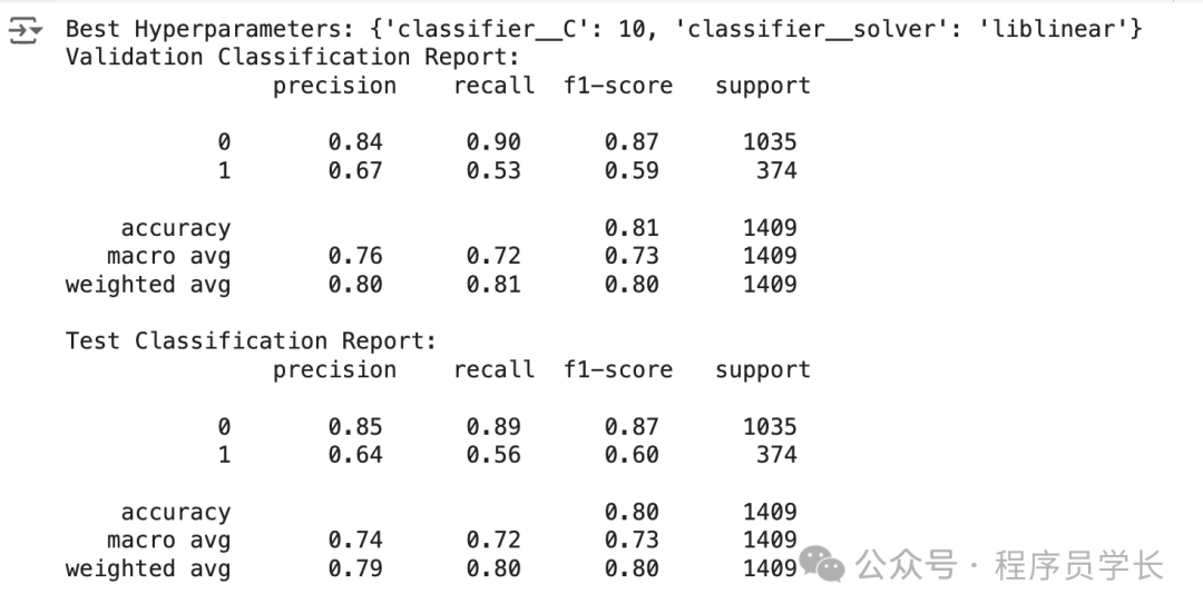
优化模型的一种方法是通过超参数优化,它会测试这些模型超参数的所有组合,以根据指标找到最佳组合。
每个模型都有一组超参数,我们可以在训练之前设置它们。
from sklearn.model_selection import GridSearchCV
# Define the logistic regression model within a pipeline
pipeline = Pipeline(steps=[
    ('preprocessor', preprocessor),
    ('classifier', LogisticRegression(max_iter=1000))
])

# Define the hyperparameters for GridSearchCV
param_grid = {
    'classifier__C': [0.1, 1, 10, 100],
    'classifier__solver': ['lbfgs', 'liblinear']
}

# Perform Grid Search with cross-validation
grid_search = GridSearchCV(pipeline, param_grid, cv=5, scoring='recall')
grid_search.fit(X_train, y_train)

# Best hyperparameters
print("Best Hyperparameters:", grid_search.best_params_)

# Evaluate on the validation set
y_val_pred = grid_search.predict(X_val)
print("Validation Classification Report:\n", classification_report(y_val, y_val_pred))

# Evaluate on the test set
y_test_pred = grid_search.predict(X_test)
print("Test Classification Report:\n", classification_report(y_test, y_test_pred))
5.部署模型
我们已经构建了机器学习模型。有了模型之后,下一步就是将其部署到生产中。让我们使用一个简单的 API 来模拟它。
首先,让我们再次开发我们的模型并将其保存为 joblib 对象。
import joblib

best_params = {'classifier__C': 10, 'classifier__solver': 'liblinear'}
logreg_model = LogisticRegression(C=best_params['classifier__C'], solver=best_params['classifier__solver'], max_iter=1000)

preprocessor = ColumnTransformer(
    transformers=[
        ('num', 'passthrough', num_features),
        ('cat', OneHotEncoder(), cat_features)])

pipeline = Pipeline(steps=[
    ('preprocessor', preprocessor),
    ('classifier', logreg_model)
])

pipeline.fit(X_train, y_train)

# Save the model
joblib.dump(pipeline, 'logreg_model.joblib')
一旦模型对象准备就绪,我们将创建一个名为 app.py 的 Python 脚本,并将以下代码放入脚本中。
from fastapi import FastAPI
from pydantic import BaseModel
import joblib
import numpy as np

# Load the logistic regression model pipeline
model = joblib.load('logreg_model.joblib')

# Define the input data for model
class CustomerData(BaseModel):
    tenure: int
    InternetService: str
    OnlineSecurity: str
    TechSupport: str
    Contract: str
    PaymentMethod: str

# Create FastAPI app
app = FastAPI()

# Define prediction endpoint
@app.post("/predict")
def predict(data: CustomerData):
    input_data = {
        'tenure': [data.tenure],
        'InternetService': [data.InternetService],
        'OnlineSecurity': [data.OnlineSecurity],
        'TechSupport': [data.TechSupport],
        'Contract': [data.Contract],        'PaymentMethod': [data.PaymentMethod]
    }

    import pandas as pd
    input_df = pd.DataFrame(input_data)

    # Make a prediction
    prediction = model.predict(input_df)

    # Return the prediction
    return {"prediction": int(prediction[0])}

if __name__ == "__main__":
    import uvicorn
    uvicorn.run(app, host="0.0.0.0", port=8000)
在命令提示符或终端中,运行以下代码。
uvicorn app:app --reload
有了上面的代码,我们已经有一个用于接受数据和创建预测的 API。
让我们在新终端中使用以下代码尝试一下。
curl -X POST "http://127.0.0.1:8000/predict" -H "Content-Type: application/json" -d "{\"tenure\": 72, \"InternetService\": \"Fiber optic\", \"OnlineSecurity\": \"Yes\", \"TechSupport\": \"Yes\", \"Contract\": \"Two year\", \"PaymentMethod\": \"Credit card (automatic)\"}"
如你所见,API 结果是一个预测值为 0(Not-Churn)的字典。你可以进一步调整代码以获得所需的结果。
最后
—
今天的分享就到这里。如果觉得近期的文章不错,请点赞,转发安排起来。
## AI大模型学习福利
作为一名热心肠的互联网老兵,我决定把宝贵的AI知识分享给大家。 至于能学习到多少就看你的学习毅力和能力了 。我已将重要的AI大模型资料包括AI大模型入门学习思维导图、精品AI大模型学习书籍手册、视频教程、实战学习等录播视频免费分享出来。
因篇幅有限,仅展示部分资料,需要点击下方链接即可前往获取
2025最新版CSDN大礼包:《AGI大模型学习资源包》免费分享
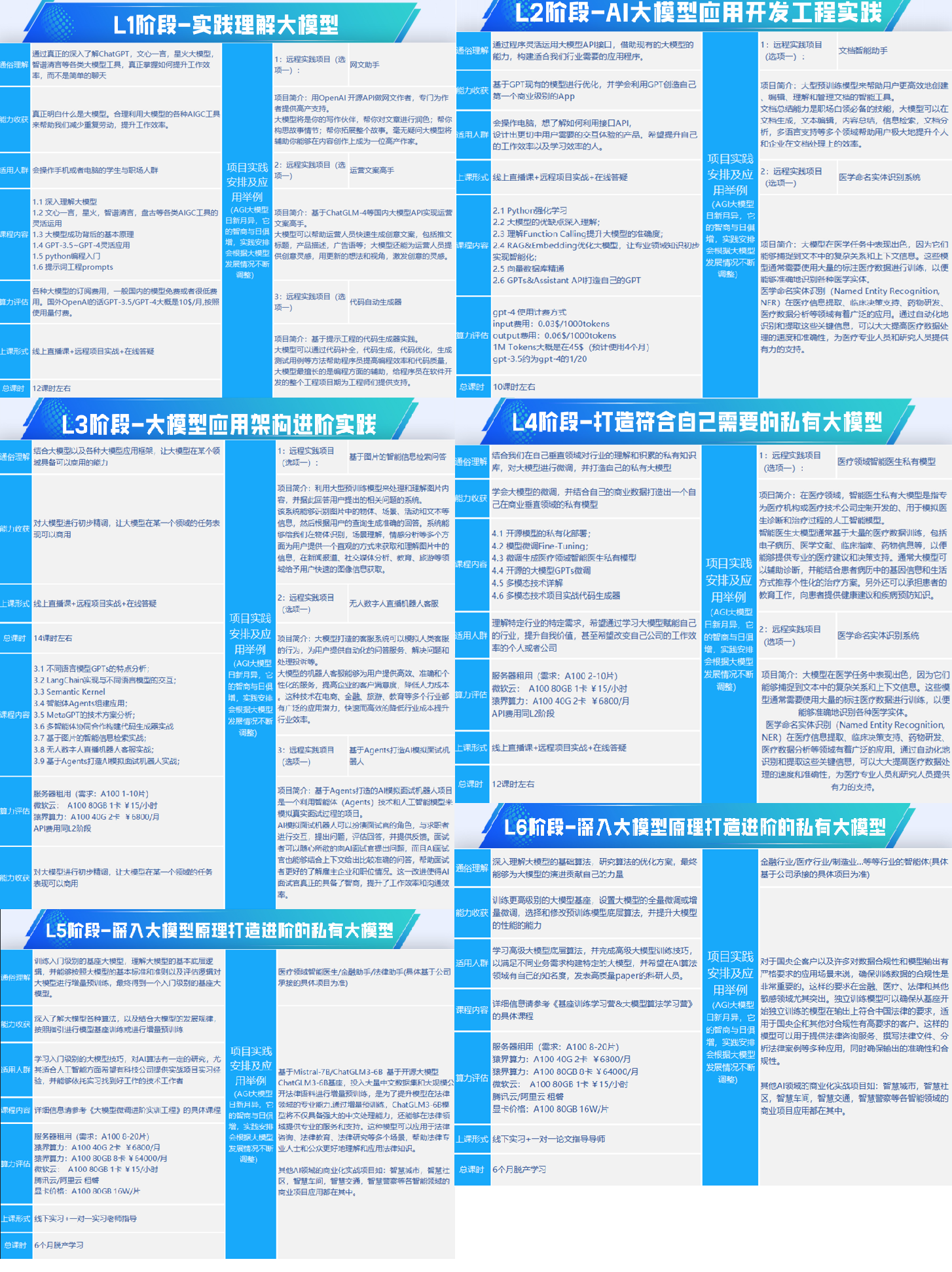
一、全套AGI大模型学习路线
AI大模型时代的学习之旅:从基础到前沿,掌握人工智能的核心技能!
因篇幅有限,仅展示部分资料,需要点击下方链接即可前往获取
2025最新版CSDN大礼包:《AGI大模型学习资源包》免费分享
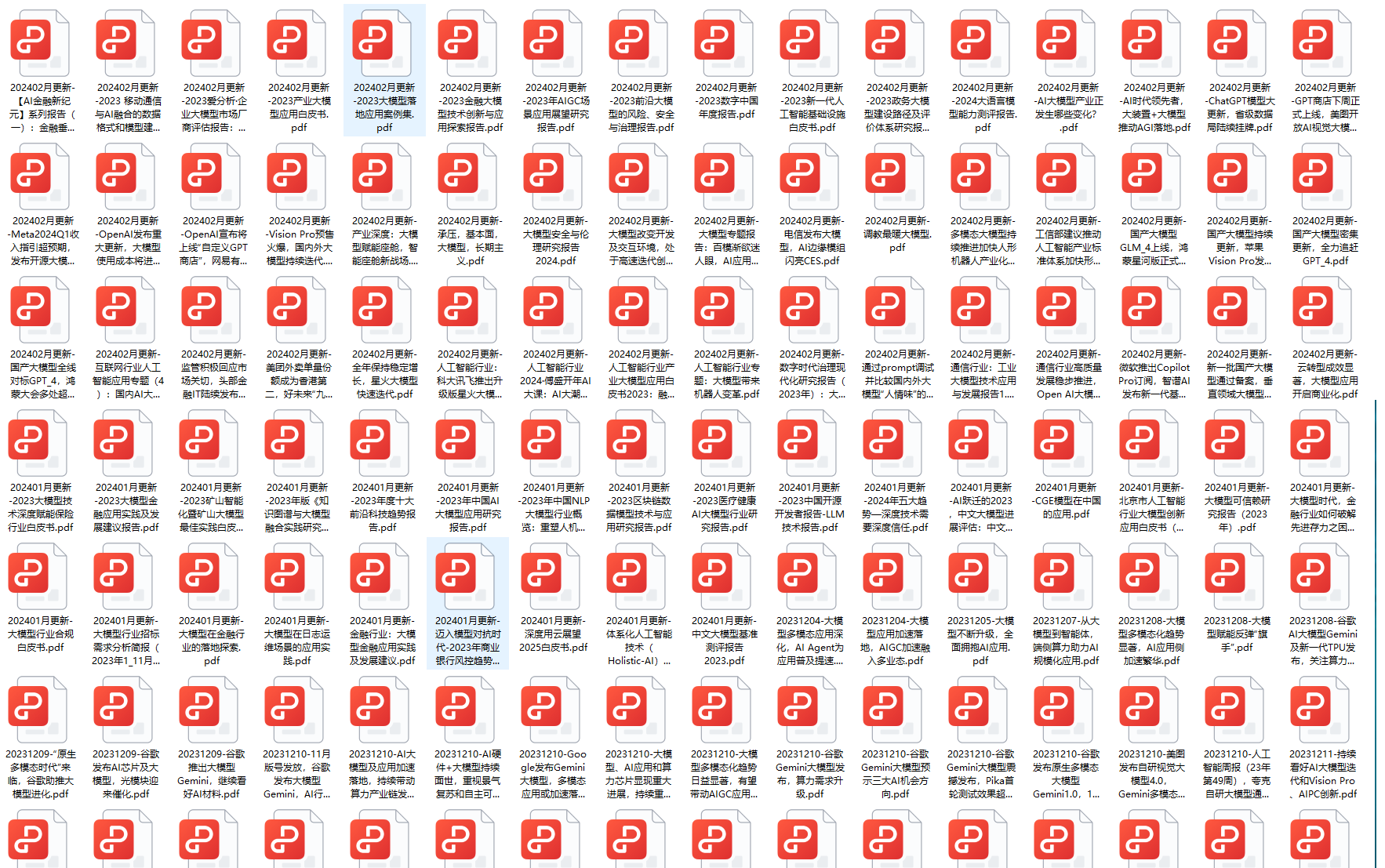
二、640套AI大模型报告合集
这套包含640份报告的合集,涵盖了AI大模型的理论研究、技术实现、行业应用等多个方面。无论您是科研人员、工程师,还是对AI大模型感兴趣的爱好者,这套报告合集都将为您提供宝贵的信息和启示。
因篇幅有限,仅展示部分资料,需要点击下方链接即可前往获取
2025最新版CSDN大礼包:《AGI大模型学习资源包》免费分享
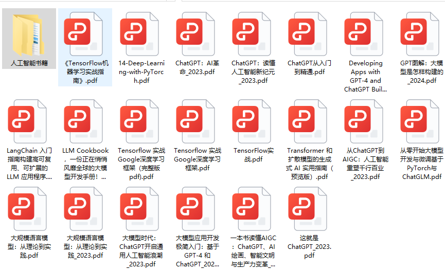
三、AI大模型经典PDF籍
随着人工智能技术的飞速发展,AI大模型已经成为了当今科技领域的一大热点。这些大型预训练模型,如GPT-3、BERT、XLNet等,以其强大的语言理解和生成能力,正在改变我们对人工智能的认识。 那以下这些PDF籍就是非常不错的学习资源。
因篇幅有限,仅展示部分资料,需要点击下方链接即可前往获取
2025最新版CSDN大礼包:《AGI大模型学习资源包》免费分享
四、AI大模型商业化落地方案

因篇幅有限,仅展示部分资料,需要点击下方链接即可前往获取
2025最新版CSDN大礼包:《AGI大模型学习资源包》免费分享
作为普通人,入局大模型时代需要持续学习和实践,不断提高自己的技能和认知水平,同时也需要有责任感和伦理意识,为人工智能的健康发展贡献力量。

有“AI”的1024 = 2048,欢迎大家加入2048 AI社区
更多推荐
 29
29 0
0- 0


 已为社区贡献125条内容

所有评论(0)