---

前言

本文主要涉及《PENet: Towards Precise and Efficient Image Guided Depth Completion》论文解读和代码理解.

---

研究背景及动机

深度补全任务：在有或无参考图像的指导下，由稀疏深度图生成密集深度图。
本文提出了一种高准确性、高实时性的深度补全网络。

---

主要创新点

1. 构造了一个双分支骨干网络（A Strong Two-branch Backbone），能够通过彩色和深度作为引导信息来进行稠密深度预测。这个架构能够利用和融合彩色和深度信息。
2. 提出一个几何卷积层（Geometric Convolutional Layer）来简化3D几何线索。
3. 设计网络来加速深度精细技术CSPN++（Dilated and Accelerated CSPN++），使其变得更加高效。

---

Geometric Convolutional Layer

为了便于理解，先介绍Geometric Convolutional Layer。

与传统卷积不同的是，Geometric Convolutional Layer会从输入中提取$(x,y,z)$位置图，与特征拼接后再进行卷积。位置图的生成方法如下：
$$Z=D,X=\frac{(u-u_0)Z}{f_x},Y=\frac{(\nu -{\nu }_0)Z}{f_y}$$
其中，$(u,v)$表示像素，$u_0$,$v_0$,$f_x$,$f_y$表示相机参数。

Geometric Convolutional Layer形成卷积前拼接特征的实现代码如下：

class GeometryFeature(nn.Module):
    def __init__(self):
        super(GeometryFeature, self).__init__()

    def forward(self, z, vnorm, unorm, h, w, ch, cw, fh, fw):
        x = z*(0.5*h*(vnorm+1)-ch)/fh
        y = z*(0.5*w*(unorm+1)-cw)/fw
        return torch.cat((x, y, z),1)

Geometric Convolutional Layer用于替换残差块中的传统卷积层，具体实现如下：

class BasicBlockGeo(nn.Module):
    expansion = 1
    __constants__ = ['downsample']

    def __init__(self, inplanes, planes, stride=1, downsample=None, groups=1,
                 base_width=64, dilation=1, norm_layer=None, geoplanes=3):
        super(BasicBlockGeo, self).__init__()

        if norm_layer is None:
            norm_layer = nn.BatchNorm2d
            #norm_layer = encoding.nn.BatchNorm2d
        if groups != 1 or base_width != 64:
            raise ValueError('BasicBlock only supports groups=1 and base_width=64')
        if dilation > 1:
            raise NotImplementedError("Dilation > 1 not supported in BasicBlock")
        # Both self.conv1 and self.downsample layers downsample the input when stride != 1
        self.conv1 = conv3x3(inplanes + geoplanes, planes, stride)
        self.bn1 = norm_layer(planes)
        self.relu = nn.ReLU(inplace=True)
        self.conv2 = conv3x3(planes+geoplanes, planes)
        self.bn2 = norm_layer(planes)
        if stride != 1 or inplanes != planes:
            downsample = nn.Sequential(
                conv1x1(inplanes+geoplanes, planes, stride),
                norm_layer(planes),
            )
        self.downsample = downsample
        self.stride = stride

    def forward(self, x, g1=None, g2=None):  # x表示输入特征，g1/g2表示第一/二次卷积前的需要拼接的几何特征
        identity = x
        if g1 is not None:
            x = torch.cat((x, g1), 1)  # 拼接几何特征
        out = self.conv1(x)
        out = self.bn1(out)
        out = self.relu(out)

        if g2 is not None:
            out = torch.cat((g2,out), 1)  # 拼接几何特征
        out = self.conv2(out)
        out = self.bn2(out)

        if self.downsample is not None:
            identity = self.downsample(x)  # 提取残差特征

        out += identity  # 残差连接
        out = self.relu(out)

        return out

---

A Strong Two-branch Backbone

整个骨干网络由 颜色主导分支（Color-dominant Branch） 和 深度主导分支（Depth-dominant Branch） 构成，每个分支均是编码器-解码器结构，由卷积层、残差块和反卷积层构成。
颜色主导分支，输入为图像+稀疏深度图，输出为CD深度图（CD-Depth）+CD置信度（CD-Confidence）。
深度主导分支，输入为CD深度图+稀疏深度图，输出为DD深度图（DD-Depth）+DD置信度（DD-Confidence）。
最终输出融合深度图（Fused Depth）：
$${\hat{D}}_f(u,v)=\frac{e^{C_{cd}(u,v)}\cdot {\hat{D}}_{cd}(u,v)+e^{C_{dd}(u,v)}\cdot {\hat{D}}_{dd}(u,v)}{e^{C_{cd}(u,v)}+e^{C_{dd}(u,v)}}$$
其中$(u,v)$表示像素，${\hat{D}}_f$表示融合深度图，${\hat{D}}_{cd}$和${\hat{D}}_{dd}$依次表示CD深度图和DD深度图，$C_{cd}$和$C_{dd}$依次表示CD置信度和DD置信度。

骨干网络的源码：

class ENet(nn.Module):
    def __init__(self, args):
        super(ENet, self).__init__()
        self.args = args
        self.geofeature = None
        self.geoplanes = 3
        if self.args.convolutional_layer_encoding == "xyz":
            self.geofeature = GeometryFeature()
        elif self.args.convolutional_layer_encoding == "std":
            self.geoplanes = 0
        elif self.args.convolutional_layer_encoding == "uv":
            self.geoplanes = 2
        elif self.args.convolutional_layer_encoding == "z":
            self.geoplanes = 1

        # rgb encoder
        self.rgb_conv_init = convbnrelu(in_channels=4, out_channels=32, kernel_size=5, stride=1, padding=2)

        self.rgb_encoder_layer1 = BasicBlockGeo(inplanes=32, planes=64, stride=2, geoplanes=self.geoplanes)
        self.rgb_encoder_layer2 = BasicBlockGeo(inplanes=64, planes=64, stride=1, geoplanes=self.geoplanes)
        self.rgb_encoder_layer3 = BasicBlockGeo(inplanes=64, planes=128, stride=2, geoplanes=self.geoplanes)
        self.rgb_encoder_layer4 = BasicBlockGeo(inplanes=128, planes=128, stride=1, geoplanes=self.geoplanes)
        self.rgb_encoder_layer5 = BasicBlockGeo(inplanes=128, planes=256, stride=2, geoplanes=self.geoplanes)
        self.rgb_encoder_layer6 = BasicBlockGeo(inplanes=256, planes=256, stride=1, geoplanes=self.geoplanes)
        self.rgb_encoder_layer7 = BasicBlockGeo(inplanes=256, planes=512, stride=2, geoplanes=self.geoplanes)
        self.rgb_encoder_layer8 = BasicBlockGeo(inplanes=512, planes=512, stride=1, geoplanes=self.geoplanes)
        self.rgb_encoder_layer9 = BasicBlockGeo(inplanes=512, planes=1024, stride=2, geoplanes=self.geoplanes)
        self.rgb_encoder_layer10 = BasicBlockGeo(inplanes=1024, planes=1024, stride=1, geoplanes=self.geoplanes)

        self.rgb_decoder_layer8 = deconvbnrelu(in_channels=1024, out_channels=512, kernel_size=5, stride=2, padding=2, output_padding=1)
        self.rgb_decoder_layer6 = deconvbnrelu(in_channels=512, out_channels=256, kernel_size=5, stride=2, padding=2, output_padding=1)
        self.rgb_decoder_layer4 = deconvbnrelu(in_channels=256, out_channels=128, kernel_size=5, stride=2, padding=2, output_padding=1)
        self.rgb_decoder_layer2 = deconvbnrelu(in_channels=128, out_channels=64, kernel_size=5, stride=2, padding=2, output_padding=1)
        self.rgb_decoder_layer0 = deconvbnrelu(in_channels=64, out_channels=32, kernel_size=5, stride=2, padding=2, output_padding=1)
        self.rgb_decoder_output = deconvbnrelu(in_channels=32, out_channels=2, kernel_size=3, stride=1, padding=1, output_padding=0)


        # depth encoder
        self.depth_conv_init = convbnrelu(in_channels=2, out_channels=32, kernel_size=5, stride=1, padding=2)

        self.depth_layer1 = BasicBlockGeo(inplanes=32, planes=64, stride=2, geoplanes=self.geoplanes)
        self.depth_layer2 = BasicBlockGeo(inplanes=64, planes=64, stride=1, geoplanes=self.geoplanes)
        self.depth_layer3 = BasicBlockGeo(inplanes=128, planes=128, stride=2, geoplanes=self.geoplanes)
        self.depth_layer4 = BasicBlockGeo(inplanes=128, planes=128, stride=1, geoplanes=self.geoplanes)
        self.depth_layer5 = BasicBlockGeo(inplanes=256, planes=256, stride=2, geoplanes=self.geoplanes)
        self.depth_layer6 = BasicBlockGeo(inplanes=256, planes=256, stride=1, geoplanes=self.geoplanes)
        self.depth_layer7 = BasicBlockGeo(inplanes=512, planes=512, stride=2, geoplanes=self.geoplanes)
        self.depth_layer8 = BasicBlockGeo(inplanes=512, planes=512, stride=1, geoplanes=self.geoplanes)
        self.depth_layer9 = BasicBlockGeo(inplanes=1024, planes=1024, stride=2, geoplanes=self.geoplanes)
        self.depth_layer10 = BasicBlockGeo(inplanes=1024, planes=1024, stride=1, geoplanes=self.geoplanes)

        # decoder
        self.decoder_layer1 = deconvbnrelu(in_channels=1024, out_channels=512, kernel_size=5, stride=2, padding=2, output_padding=1)
        self.decoder_layer2 = deconvbnrelu(in_channels=512, out_channels=256, kernel_size=5, stride=2, padding=2, output_padding=1)
        self.decoder_layer3 = deconvbnrelu(in_channels=256, out_channels=128, kernel_size=5, stride=2, padding=2, output_padding=1)
        self.decoder_layer4 = deconvbnrelu(in_channels=128, out_channels=64, kernel_size=5, stride=2, padding=2, output_padding=1)
        self.decoder_layer5 = deconvbnrelu(in_channels=64, out_channels=32, kernel_size=5, stride=2, padding=2, output_padding=1)

        self.decoder_layer6 = convbnrelu(in_channels=32, out_channels=2, kernel_size=3, stride=1, padding=1)
        self.softmax = nn.Softmax(dim=1)
        self.pooling = nn.AvgPool2d(kernel_size=2)
        self.sparsepooling = SparseDownSampleClose(stride=2)
        '''
        对稀疏数据进行下采样。通过使用一个大值 (self.large_number) 对掩码为 0 的位置进行标记，这样在池化操作中这些位置不会干扰计算。池化操作完成后，再将这些位置的值恢复到适当的状态。
        class SparseDownSampleClose(nn.Module):  # 利用掩码对稀疏数据进行池化的操作
		    def __init__(self, stride):
		        super(SparseDownSampleClose, self).__init__()
		        self.pooling = nn.MaxPool2d(stride, stride)
		        self.large_number = 600
		    def forward(self, d, mask):
		        encode_d = - (1-mask)*self.large_number - d  # 计算了一个编码版本的d，其中掩码为0的位置被赋值为-self.large_number，这样在后续池化的过程中不影响结果
		
		        d = - self.pooling(encode_d)  # 对编码后的d进行池化操作，将池化区域内最大值提取出来并忽略掩码为0的位置
		        mask_result = self.pooling(mask)  # 对mask进行池化操作，以配合池化后的数据
		        d_result = d - (1-mask_result)*self.large_number  # 通过从池化后的d中减去填充位置的值（这些位置在池化前被标记为 -self.large_number），得到最终的下采样结果
		
		        return d_result, mask_result
        '''

        weights_init(self)

    def forward(self, input):
        #independent input
        rgb = input['rgb']  # 图像，(B, 3, H, W)
        d = input['d']  # 稀疏深度图，(B, 1, H, W)

        position = input['position']  # 归一化后的像素坐标，（B, 2, H, W）
        K = input['K']  # 内参矩阵，（B, 3， 3）
        unorm = position[:, 0:1, :, :]
        vnorm = position[:, 1:2, :, :]

        f352 = K[:, 1, 1]  # fv,v方向上的焦距
        f352 = f352.unsqueeze(1)
        f352 = f352.unsqueeze(2)
        f352 = f352.unsqueeze(3)
        c352 = K[:, 1, 2]  # cv，v方向上的偏移
        c352 = c352.unsqueeze(1)
        c352 = c352.unsqueeze(2)
        c352 = c352.unsqueeze(3)
        f1216 = K[:, 0, 0]  # fu，u方向上的焦距
        f1216 = f1216.unsqueeze(1)
        f1216 = f1216.unsqueeze(2)
        f1216 = f1216.unsqueeze(3)
        c1216 = K[:, 0, 2]  # cu，u方向上的偏移
        c1216 = c1216.unsqueeze(1)
        c1216 = c1216.unsqueeze(2)
        c1216 = c1216.unsqueeze(3)

        vnorm_s2 = self.pooling(vnorm)  # stride=2^(2-1)时，v方向归一化坐标
        vnorm_s3 = self.pooling(vnorm_s2)
        vnorm_s4 = self.pooling(vnorm_s3)
        vnorm_s5 = self.pooling(vnorm_s4)
        vnorm_s6 = self.pooling(vnorm_s5)

        unorm_s2 = self.pooling(unorm)  # stride=2^(2-1)时，u方向归一化坐标
        unorm_s3 = self.pooling(unorm_s2)
        unorm_s4 = self.pooling(unorm_s3)
        unorm_s5 = self.pooling(unorm_s4)
        unorm_s6 = self.pooling(unorm_s5)

        valid_mask = torch.where(d>0, torch.full_like(d, 1.0), torch.full_like(d, 0.0))
        d_s2, vm_s2 = self.sparsepooling(d, valid_mask)  # stride=2^(2-1)时，稀疏的d和valid mask
        d_s3, vm_s3 = self.sparsepooling(d_s2, vm_s2)
        d_s4, vm_s4 = self.sparsepooling(d_s3, vm_s3)
        d_s5, vm_s5 = self.sparsepooling(d_s4, vm_s4)
        d_s6, vm_s6 = self.sparsepooling(d_s5, vm_s5)        

        geo_s1 = None
        geo_s2 = None
        geo_s3 = None
        geo_s4 = None
        geo_s5 = None
        geo_s6 = None

        if self.args.convolutional_layer_encoding == "xyz":
        	# 形成Geometric Convolutional Layer卷积前的拼接特征
            geo_s1 = self.geofeature(d, vnorm, unorm, 352, 1216, c352, c1216, f352, f1216)
            geo_s2 = self.geofeature(d_s2, vnorm_s2, unorm_s2, 352 / 2, 1216 / 2, c352, c1216, f352, f1216)
            geo_s3 = self.geofeature(d_s3, vnorm_s3, unorm_s3, 352 / 4, 1216 / 4, c352, c1216, f352, f1216)
            geo_s4 = self.geofeature(d_s4, vnorm_s4, unorm_s4, 352 / 8, 1216 / 8, c352, c1216, f352, f1216)
            geo_s5 = self.geofeature(d_s5, vnorm_s5, unorm_s5, 352 / 16, 1216 / 16, c352, c1216, f352, f1216)
            geo_s6 = self.geofeature(d_s6, vnorm_s6, unorm_s6, 352 / 32, 1216 / 32, c352, c1216, f352, f1216)
        elif self.args.convolutional_layer_encoding == "uv":
            geo_s1 = torch.cat((vnorm, unorm), dim=1)
            geo_s2 = torch.cat((vnorm_s2, unorm_s2), dim=1)
            geo_s3 = torch.cat((vnorm_s3, unorm_s3), dim=1)
            geo_s4 = torch.cat((vnorm_s4, unorm_s4), dim=1)
            geo_s5 = torch.cat((vnorm_s5, unorm_s5), dim=1)
            geo_s6 = torch.cat((vnorm_s6, unorm_s6), dim=1)
        elif self.args.convolutional_layer_encoding == "z":
            geo_s1 = d
            geo_s2 = d_s2
            geo_s3 = d_s3
            geo_s4 = d_s4
            geo_s5 = d_s5
            geo_s6 = d_s6

        #embeded input
        #rgb = input[:, 0:3, :, :]
        #d = input[:, 3:4, :, :]

        # b 1 352 1216
        rgb_feature = self.rgb_conv_init(torch.cat((rgb, d), dim=1))
        rgb_feature1 = self.rgb_encoder_layer1(rgb_feature, geo_s1, geo_s2) # b 32 176 608
        rgb_feature2 = self.rgb_encoder_layer2(rgb_feature1, geo_s2, geo_s2) # b 32 176 608
        rgb_feature3 = self.rgb_encoder_layer3(rgb_feature2, geo_s2, geo_s3) # b 64 88 304
        rgb_feature4 = self.rgb_encoder_layer4(rgb_feature3, geo_s3, geo_s3) # b 64 88 304
        rgb_feature5 = self.rgb_encoder_layer5(rgb_feature4, geo_s3, geo_s4) # b 128 44 152
        rgb_feature6 = self.rgb_encoder_layer6(rgb_feature5, geo_s4, geo_s4) # b 128 44 152
        rgb_feature7 = self.rgb_encoder_layer7(rgb_feature6, geo_s4, geo_s5) # b 256 22 76
        rgb_feature8 = self.rgb_encoder_layer8(rgb_feature7, geo_s5, geo_s5) # b 256 22 76
        rgb_feature9 = self.rgb_encoder_layer9(rgb_feature8, geo_s5, geo_s6) # b 512 11 38
        rgb_feature10 = self.rgb_encoder_layer10(rgb_feature9, geo_s6, geo_s6) # b 512 11 38

        rgb_feature_decoder8 = self.rgb_decoder_layer8(rgb_feature10)
        rgb_feature8_plus = rgb_feature_decoder8 + rgb_feature8

        rgb_feature_decoder6 = self.rgb_decoder_layer6(rgb_feature8_plus)
        rgb_feature6_plus = rgb_feature_decoder6 + rgb_feature6

        rgb_feature_decoder4 = self.rgb_decoder_layer4(rgb_feature6_plus)
        rgb_feature4_plus = rgb_feature_decoder4 + rgb_feature4

        rgb_feature_decoder2 = self.rgb_decoder_layer2(rgb_feature4_plus)
        rgb_feature2_plus = rgb_feature_decoder2 + rgb_feature2   # b 32 176 608

        rgb_feature_decoder0 = self.rgb_decoder_layer0(rgb_feature2_plus)
        rgb_feature0_plus = rgb_feature_decoder0 + rgb_feature

        rgb_output = self.rgb_decoder_output(rgb_feature0_plus)
        rgb_depth = rgb_output[:, 0:1, :, :]
        rgb_conf = rgb_output[:, 1:2, :, :]

        # -----------------------------------------------------------------------
        # mask = torch.where(d>0, torch.full_like(d, 1.0), torch.full_like(d, 0.0))
        # input = torch.cat([d, mask], 1)

        sparsed_feature = self.depth_conv_init(torch.cat((d, rgb_depth), dim=1))
        sparsed_feature1 = self.depth_layer1(sparsed_feature, geo_s1, geo_s2)# b 32 176 608
        sparsed_feature2 = self.depth_layer2(sparsed_feature1, geo_s2, geo_s2) # b 32 176 608

        sparsed_feature2_plus = torch.cat([rgb_feature2_plus, sparsed_feature2], 1)
        sparsed_feature3 = self.depth_layer3(sparsed_feature2_plus, geo_s2, geo_s3) # b 64 88 304
        sparsed_feature4 = self.depth_layer4(sparsed_feature3, geo_s3, geo_s3) # b 64 88 304

        sparsed_feature4_plus = torch.cat([rgb_feature4_plus, sparsed_feature4], 1)
        sparsed_feature5 = self.depth_layer5(sparsed_feature4_plus, geo_s3, geo_s4) # b 128 44 152
        sparsed_feature6 = self.depth_layer6(sparsed_feature5, geo_s4, geo_s4) # b 128 44 152

        sparsed_feature6_plus = torch.cat([rgb_feature6_plus, sparsed_feature6], 1)
        sparsed_feature7 = self.depth_layer7(sparsed_feature6_plus, geo_s4, geo_s5) # b 256 22 76
        sparsed_feature8 = self.depth_layer8(sparsed_feature7, geo_s5, geo_s5) # b 256 22 76

        sparsed_feature8_plus = torch.cat([rgb_feature8_plus, sparsed_feature8], 1)
        sparsed_feature9 = self.depth_layer9(sparsed_feature8_plus, geo_s5, geo_s6) # b 512 11 38
        sparsed_feature10 = self.depth_layer10(sparsed_feature9, geo_s6, geo_s6) # b 512 11 38

        # -----------------------------------------------------------------------------------------

        fusion1 = rgb_feature10 + sparsed_feature10  # 将颜色主导分支的特征融合至深度主导分支
        decoder_feature1 = self.decoder_layer1(fusion1)

        fusion2 = sparsed_feature8 + decoder_feature1
        decoder_feature2 = self.decoder_layer2(fusion2)

        fusion3 = sparsed_feature6 + decoder_feature2
        decoder_feature3 = self.decoder_layer3(fusion3)

        fusion4 = sparsed_feature4 + decoder_feature3
        decoder_feature4 = self.decoder_layer4(fusion4)

        fusion5 = sparsed_feature2 + decoder_feature4
        decoder_feature5 = self.decoder_layer5(fusion5)

        depth_output = self.decoder_layer6(decoder_feature5)
        d_depth, d_conf = torch.chunk(depth_output, 2, dim=1)

        # 融合深度图
        rgb_conf, d_conf = torch.chunk(self.softmax(torch.cat((rgb_conf, d_conf), dim=1)), 2, dim=1)
        output = rgb_conf*rgb_depth + d_conf*d_depth

        if(self.args.network_model == 'e'):
            return rgb_depth, d_depth, output
        elif(self.args.dilation_rate == 1):
            return torch.cat((rgb_feature0_plus, decoder_feature5),1), output
        elif (self.args.dilation_rate == 2):
            return torch.cat((rgb_feature0_plus, decoder_feature5), 1), torch.cat((rgb_feature2_plus, decoder_feature4),1), output
        elif (self.args.dilation_rate == 4):
            return torch.cat((rgb_feature0_plus, decoder_feature5), 1), torch.cat((rgb_feature2_plus, decoder_feature4),1),\
                   torch.cat((rgb_feature4_plus, decoder_feature3), 1), output

---

Dilated and Accelerated CSPN++

本章将以此介绍SPN、CSPN、CSPN++和Dilated and Accelerated CSPN++。

参考博客 讲解的非常细致，本文描述相关内容时会更为精炼。

SPN

SPN全称Spatial Propagation Networks，是亲和矩阵的“开山之作”。
空间扩散的线性传播
通过空间传播网络应用线性变换，矩阵以行/列路径在四个固定方向上扫描：从左到右，从上到下，还有它们的反方向（从下到上、从右到左）。本文以从左到右的方向为例讨论，其他方向以同样的方式独立处理。
假设$X$和$H$为两个$n\times n$二维图，维度与空间传播前后的矩阵完全相同，$x_t$和$h_t$表示两二维图的第$t$列，每列有$n\times 1$个元素。使用$n\times n$线性变换矩阵$w_t$在相邻列之间从左到右线性传播信息：
$$h_t=(I-d_t)x_t+w_t{h}_{t-1},t\in [2,n]$$
其中$I$为$n\times n$单位矩阵，初始条件$h_1=x_1$，$d_t(i,i)$是一个对角阵，其中第$(i,i)$个元素是$w_t$的第$i$行除第$i$列的所有元素之和：
$$d_t(i,i)=\sum _{j=1,j\ne i}^n{w}_t(i,j)$$
矩阵$H$中 { h t ∈ H , t ∈ [ 1 , n ] } \{ h_{t}\in H,t\in[1,n] \} {ht​∈H,t∈[1,n]}逐列递归更新。对于每一列$h_t$，$h_t$是前一列$h_{t-1}$和$X$中对应列$x_t$的线性组合。

以$3\times 3$为例，进行迭代演示
$$x_1=\left[\begin{array}{c}{x}_{11}\\ x_{21}\\ x_{31}\end{array}\right],h_1=x_1=\left[\begin{array}{c}{x}_{11}\\ x_{21}\\ x_{31}\end{array}\right]$$
$$x_2=\left[\begin{array}{c}{x}_{12}\\ x_{22}\\ x_{32}\end{array}\right],h_2=(I-d_2)x_2+w_2{h}_1=(\left[\begin{array}{ccc}1& 0& 0\\ 0& 1& 0\\ 0& 0& 1\end{array}\right]-\left[\begin{array}{ccc}{w}_2(1,2)+w_2(1,3)& 0& 0\\ 0& w_2(2,1)+w_2(2,3)& 0\\ 0& 0& w_2(3,1)+w_2(3,2)\end{array}\right])\left[\begin{array}{c}{x}_{12}\\ x_{22}\\ x_{32}\end{array}\right]+\left[\begin{array}{ccc}{w}_2(1,1)& w_2(1,2)& w_2(1,3)\\ w_2(2,1)& w_2(2,2)& w_2(2,3)\\ w_2(3,1)& w_2(3,2)& w_2(3,3)\end{array}\right]\left[\begin{array}{c}{h}_{11}\\ h_{21}\\ h_{31}\end{array}\right]$$
$$x_3=\left[\begin{array}{c}{x}_{13}\\ x_{23}\\ x_{33}\end{array}\right],h_3=(I-d_3)x_3+w_3{h}_2=(\left[\begin{array}{ccc}1& 0& 0\\ 0& 1& 0\\ 0& 0& 1\end{array}\right]-\left[\begin{array}{ccc}{w}_3(1,2)+w_3(1,3)& 0& 0\\ 0& w_3(2,1)+w_3(2,3)& 0\\ 0& 0& w_3(3,1)+w_3(3,2)\end{array}\right])\left[\begin{array}{c}{x}_{13}\\ x_{23}\\ x_{33}\end{array}\right]+\left[\begin{array}{ccc}{w}_3(1,1)& w_3(1,2)& w_3(1,3)\\ w_3(2,1)& w_3(2,2)& w_3(2,3)\\ w_3(3,1)& w_3(3,2)& w_3(3,3)\end{array}\right]\left[\begin{array}{c}{h}_{12}\\ h_{22}\\ h_{32}\end{array}\right]$$

递归扫描完成后，更新后的二维矩阵$H$可展开表示：
$$H_v=\left[\begin{array}{ccccc}I& 0& \dots & \dots & 0\\ w_2& {\lambda }_2& 0& \dots & \dots \\ w_3{w}_2& w_3{\lambda }_2& {\lambda }_3& \dots & \dots \\ \dots & \dots & \dots & \dots & \dots \\ \dots & \dots & \dots & \dots & {\lambda }_n\end{array}\right]X_v=G{X}_v$$
$H_v$和$X_v$分别是$H$和$X$的矢量化展开版本，形状为$n^2\times 1$，即$H_v=[h_1^T,h_2^T,\dots ,h_n^T{]}^T$和$X_v=[x_1^T,x_2^T,\dots ,x_n^T{]}^T$。其他参数${\lambda }_t,w_t,d_t,I(t\in [2,n])$皆为形状为$n\times n$的子矩阵，其中${\lambda }_t=I-d_t$。

以$3\times 3$为例，进行验证演示
$$H_v=\left[\begin{array}{c}{h}_1\\ h_2\\ h_3\end{array}\right],G=\left[\begin{array}{ccc}I& 0& 0\\ w_2& {\lambda }_2& 0\\ w_3{w}_2& w_3{\lambda }_2& {\lambda }_3\end{array}\right],X_v=\left[\begin{array}{c}{x}_1\\ x_2\\ x_3\end{array}\right]$$
$$h_1=I{x}_1$$
$$h_2=w_2{x}_1+{\lambda }_2{x}_2=w_2{h}_1+(I-d_2)x_2$$
$$h_3=w_3{w}_2{x}_1+w_3{\lambda }_2{x}_2+{\lambda }_3{x}_3=w_3{w}_2{h}_1+w_3(I-d_2)x_2+(I-d_3)x_3=w_3{h}_2+(I-d_3)x_3$$

定理1
G中每一行元素的和等于1（单位矩阵）。推导详见原文。
定理2
将二维矩阵的演化定义为时间序列 { U } T \{U\}_T {U}T​，其中$U(T=1)=U_1$为初始状态。当任意两个相邻状态之间的变换关系符合$G$时：$$U_{T+1}=G{U}_T$$
令：
$$G=(I-D+A)$$
$$D=\left[\begin{array}{ccccc}0& 0& \dots & \dots & 0\\ 0& d_2& 0& \dots & \dots \\ 0& 0& d_3& \dots & \dots \\ \dots & \dots & \dots & \dots & \dots \\ \dots & \dots & \dots & \dots & d_n\end{array}\right]$$
$$A=\left[\begin{array}{ccccc}0& 0& \dots & \dots & 0\\ w_2& 0& 0& \dots & \dots \\ w_3{w}_2& w_3{\lambda }_2& 0& \dots & \dots \\ \dots & \dots & \dots & \dots & \dots \\ \dots & \dots & \dots & \dots & 0\end{array}\right]$$
$$L=D-A$$
其中$L$是拉普拉斯矩阵（Laplacian Matrix）。$D$是度矩阵（Degree Matrix）。$A$是邻接矩阵（Adjacency Matrix），后面也称为亲和矩阵（Affinity Matrix）。

拉普拉斯矩阵（Laplacian matrix）是图论中的一种重要矩阵表示，与图的性质有紧密的联系。对于给定的无向图G，其拉普拉斯矩阵通常定义为度矩阵（Degree matrix）与邻接矩阵（Adjacency matrix）之差。
度矩阵（Degree matrix）是一个对角矩阵，其主对角线上的元素表示对应顶点的度数。对于一个具有$n$个顶点的图M，其度矩阵D是一个$n\times n$的矩阵，其中$D(i,j)$是顶点$i$的度数，即与顶点$i$相连的边的数量。
邻接矩阵（Adjacency matrix）是表示图中顶点之间相邻关系的矩阵。对于一个具有$n$个顶点的图M，其邻接矩阵是一个$n\times n$的矩阵A，其中$A(i,j)$表示顶点$i$和顶点$j$之间的边的权重（即这里的亲和值）。

从而可以推导出，这个时间序列是一个用偏微分方程表示的扩散过程：
$$U_{T+1}=(I-D+A)U_T=(I-L)U_T$$
$$U_{T+1}-U_T=-L{U}_T$$
$${\delta }_{T}U=-LU$$
定理2表明了空间扩散的线性传播的本质：它是一个标准的扩散过程，其中$L$定义了空间传播，$A$是亲和矩阵，描述了任意两点之间的相似性。因此学习亲和矩阵$A$相当于学习变换矩阵$w_t$。
学习基于数据驱动的亲和矩阵
由于亲和矩阵表示特定输入的成对相似性，它应该以该输入内容为条件(即，不同的输入图像应该具有不同的亲和矩阵)。论文没有将$w_t$矩阵设置为模块的固定参数，而是将其设计为深度 CNN 的输出，可以直接以输入图像为条件。
一种简单的方法是将深度CNN的输出设置为与输入矩阵使用相同的大小。当输入有c个通道(例如,一幅RGB图像有c = 3)时，输出需要n × c × 4个通道(每个通道每个像素有n个来自前一行/列的连接,有4个不同的方向)。显然，这是太多的(例如,一个128 × 128 × 16的特征图需要128 × 128 × 8192的输出)无法在现实世界的系统中实现。而不是使用相邻行/列之间的全连接，我们证明了某些局部连接，对应于稀疏的行/列变换矩阵，也可以形成密集连接的亲和力。具体来说，我们引入( a )单向连接和( b )三向连接作为实现方程的两种不同方式。

单向连接使每个像素只能连接到前一行/列的一个像素。它相当于一维(1D)线性循环传播，将每一行/列作为一维序列独立扫描。令$x_{k,t}$和$h_{k,t}$表示为第$t$列的第$k$行个像素，其中单向连接的从左到右的传播为：
$$h_{k,t}=(1-p_{k,t})\cdot x_{k,t}+p_{k,t}\cdot h_{k,t-1}$$
其中，$p_{k,t}$为标量权重，表示在$(k,t-1)$和$(k,t)$像素之间的传播强度。等价于$w_t$为对角矩阵，其由元素$p_{k,t},k\in [1,n]$组成。
三向连接允许每个像素连接到前一行/列的三个像素，即前一列的左上、中、下像素，用于从左到右的传播方向：
$$h_{k,t}=\left(1-\sum _{k\in \mathbb{N}}{p}_{k,t}\right)x_{k,t}+\sum _{k\in \mathbb{N}}{p}_{k,t}{h}_{k,t-1}$$
其中$\mathbb{N}$表示三个像素的集合，等价于$w_t$为三对角矩阵，其中$p_{:,k},k\in \mathbb{N}$构成每一行/列的三个非零元素。
与亲和矩阵的关系
单向连接构成一个备用亲和矩阵，因为$A$的每个子矩阵仅沿其对角线有非零元素，所以若干个单独的对角矩阵相乘也会得到一个对角矩阵，稀疏矩阵。
三向连接可以通过几个不同的三对角矩阵$w_t$相乘形成一个相对稠密的$A$。这意味着像素可以被稠密和全局地关联，通过简单地将空间传播过程中每个像素的连接数从一个增加到三个。
如上图所示，单向连接的传播被限制在单行，而三向连接可以将区域扩展到关于每个方向的三角2D平面。四个方向的汇总导致了所有像素之间的密集连接.

定理3
令${\left\{p_{t,k}^K\right\}}_{k\in \mathbb{N}}$为$w_t$的权重，则当${\sum }_{k\in \mathbb{N}}\left|p_{t,k}^K\right|\le 1$时，模型是稳定的。推导详见原文。
定理3表明，通过正则化隐藏层中每个像素的所有权值，使其绝对值之和小于1，可以保持线性传播模型的稳定性。
实现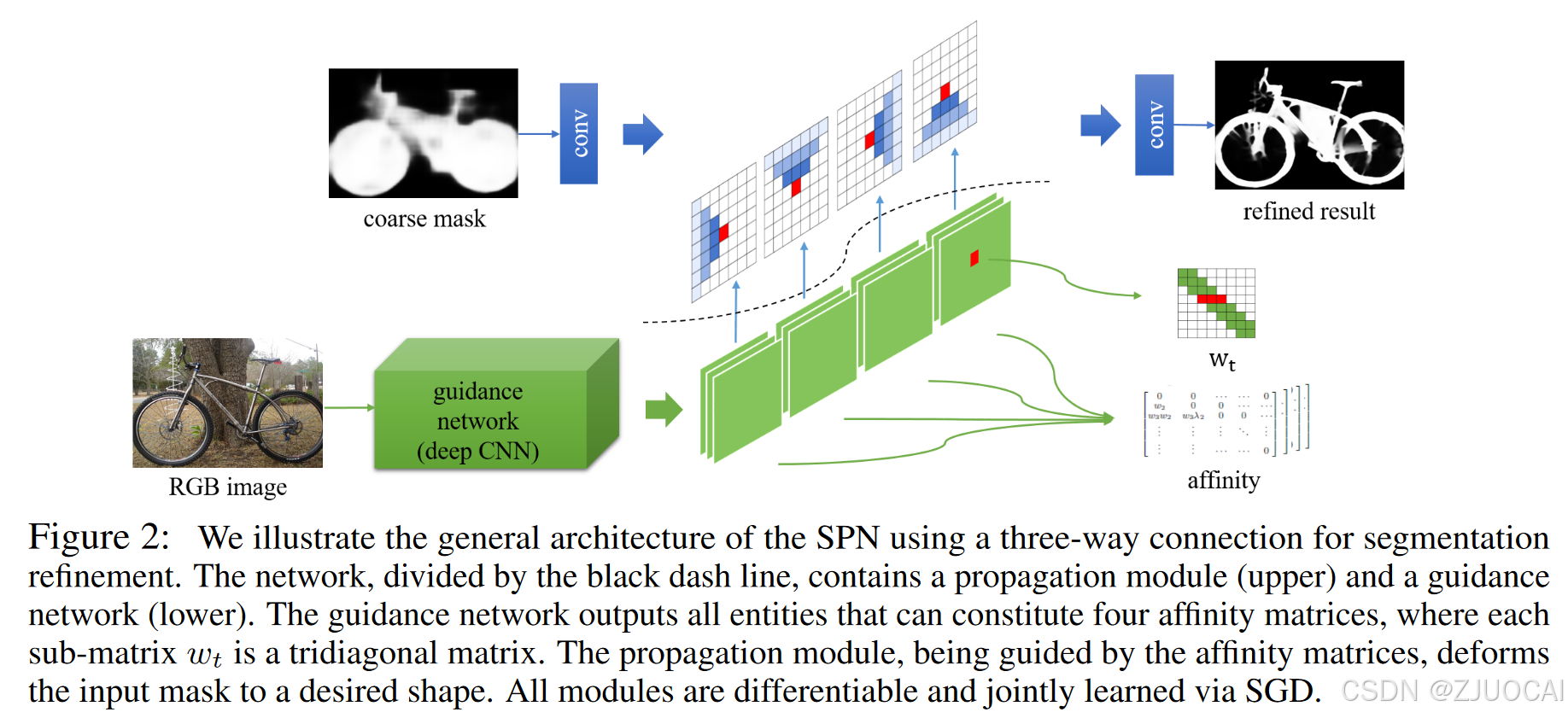

如上图所示，整个架构由黑色虚线分割，分为两部分：

1. 引导网络（下）：引导网络输出可以构成四个亲和矩阵，其中每个子矩阵$w_t$是一个三对角矩阵。引导网络将任何有助于学习关联矩阵的二维矩阵(例如，典型的RGB图像)作为输入。它输出的是构成变换矩阵$w_t$的所有权值（也就是提供亲和矩阵）。
2. 传播模块（上）：以需要传播的二维图(如粗分割 mask)和引导网络生成的权值作为输入。假设我们有一个大小为n × n × c的图输入到传播模块中，引导网络需要输出一个尺寸为n × n × c × (3 × 4)的权值图，即输入图中的每个像素每个方向对应3个标量权值，共4个方向。传播模块包含4个独立的隐藏层，用于4个不同的方向，其中每一层使用$h_{k,t}=\left(1-{\sum }_{k\in \mathbb{N}}{p}_{k,t}\right)x_{k,t}+{\sum }_{k\in \mathbb{N}}{p}_{k,t}{h}_{k,t-1}$将输入图与其各自的权重图结合起来。

代码
官方代码
引导网络输出大小为H × W × (C × 3权重× 4个方向)的张量。我们需要将张量转换为三对角矩阵，这样当我们执行点积时，它将对应于前一行/列中三个相邻像素的权重。

    def to_tridiagonal_multidim(self, w):
        # this function converts the weight vectors to a tridiagonal matrix
        
        N,W,C,D = w.size()
        
        # normalize the weights to stabilize the model
        tmp_w = w / torch.sum(torch.abs(w),dim=3).unsqueeze(-1)
        tmp_w = tmp_w.unsqueeze(2).expand([N,W,W,C,D])
        
        # three identity matrices, one normal, one shifted left and the other shifted right
        eye_a = Variable(torch.diag(torch.ones(W-1).cuda(),diagonal=-1))
        eye_b = Variable(torch.diag(torch.ones(W).cuda(),diagonal=0))
        eye_c = Variable(torch.diag(torch.ones(W-1).cuda(),diagonal=1))

        tmp_eye_a = eye_a.unsqueeze(-1).unsqueeze(0).expand([N,W,W,C])
        a = tmp_w[:,:,:,:,0] * tmp_eye_a
        tmp_eye_b = eye_b.unsqueeze(-1).unsqueeze(0).expand([N,W,W,C])
        b = tmp_w[:,:,:,:,1] * tmp_eye_b
        tmp_eye_c = eye_c.unsqueeze(-1).unsqueeze(0).expand([N,W,W,C])
        c = tmp_w[:,:,:,:,2] * tmp_eye_c

        return a+b+c

前向传播代码片段：

def forward(self, x, coarse_segmentation):
        # ...
        w_x1 = conv_x1_flat.view(N,H,W,four_directions//3,3) # N, H, W, 32, 3
        w_y1 = conv_y1_flat.view(N,H,W,four_directions//3,3) # N, H, W, 32, 3
        w_x2 = conv_x2_flat.view(N,H,W,four_directions//3,3) # N, H, W, 32, 3
        w_y2 = conv_y2_flat.view(N,H,W,four_directions//3,3) # N, H, W, 32, 3

        rnn_h1 = Variable(torch.zeros((N, H, W, four_directions//3)).cuda())
        rnn_h2 = Variable(torch.zeros((N, H, W, four_directions//3)).cuda())
        rnn_h3 = Variable(torch.zeros((N, H, W, four_directions//3)).cuda())
        rnn_h4 = Variable(torch.zeros((N, H, W, four_directions//3)).cuda())

        x_t = self.coarse_conv_in(coarse_segmentation).permute(0,2,3,1)
        
        
        # horizontal
        for i in range(W):
            #left to right
            tmp_w = w_x1[:,:,i,:,:]  # N, H, 1, 32, 3 
            tmp_w = self.to_tridiagonal_multidim(tmp_w) # N, H, W, 32 
            # tmp_x = x_t[:,:,i,:].unsqueeze(1)
            # tmp_x = tmp_x.expand([batch, W, H, 32])
            if i == 0 :
                w_h_prev = 0
            else:
                w_h_prev = torch.sum(tmp_w * rnn_h1[:,:,i-1,:].clone().unsqueeze(1).expand([N, W, H, 32]),dim=2)


            w_x_curr = (1 - torch.sum(tmp_w, dim=2)) * x_t[:,:,i,:]

            rnn_h1[:,:,i,:] = w_x_curr + w_h_prev


            #right to left
            # tmp_w = w_x1[:,:,i,:,:]  # N, H, 1, 32, 3 
            # tmp_w = to_tridiagonal_multidim(tmp_w)

            if i == 0 :
                w_h_prev = 0
            else:
                w_h_prev = torch.sum(tmp_w * rnn_h2[:,:,W - i,:].clone().unsqueeze(1).expand([N, W, H, 32]),dim=2)
   

            w_x_curr = (1 - torch.sum(tmp_w, dim=2)) * x_t[:,:,W - i-1,:]
            rnn_h2[:,:,W - i-1,:] = w_x_curr + w_h_prev 

        w_y1_T = w_y1.transpose(1,2)
        x_t_T = x_t.transpose(1,2)

        for i in range(H):
            # up to down
            tmp_w = w_y1_T[:,:,i,:,:]  # N, W, 1, 32, 3 
            tmp_w = self.to_tridiagonal_multidim(tmp_w) # N, W, H, 32 

            if i == 0 :
                w_h_prev = 0
            else:
                w_h_prev = torch.sum(tmp_w * rnn_h3[:,:,i-1,:].clone().unsqueeze(1).expand([N, H, W, 32]),dim=2)
            
            w_x_curr = (1 - torch.sum(tmp_w, dim=2)) * x_t_T[:,:,i,:]
            rnn_h3[:,:,i,:] = w_x_curr + w_h_prev

            # down to up
            if i == 0 :
                w_h_prev = 0
            else:
                w_h_prev = torch.sum(tmp_w * rnn_h4[:,:,H - i,:].clone().unsqueeze(1).expand([N, H, W, 32]),dim=2)
            
            w_x_curr = (1 - torch.sum(tmp_w, dim=2)) * x_t[:,:,H-i-1,:]
            rnn_h4[:,:,H-i-1,:] = w_x_curr + w_h_prev  

        rnn_h3 = rnn_h3.transpose(1,2)
        rnn_h4 = rnn_h4.transpose(1,2)
        # ...

CSPN

CSPN模块是一种简单高效的线性传播模型，采用循环卷积运算的方式进行传播，通过深度卷积神经网络CNN学习相邻像素之间的亲和矩阵。与空间传播网络SPN相比，CSPN在实践中速度提高了2到5倍，获得了更高的精度。
CSPN认为深度补全任务需要考虑三个重要的属性：

1. 深度保持，即保持稀疏点处的深度值；
2. 结构对齐，即估计深度图中的边缘和目标边界等详细结构与给定图像对齐；
3. 过渡平滑，即稀疏点与其邻域之间的深度过渡要平滑。

CSPN
给定一张深度图$D_o\in {\mathbf{R}}^{m\times n}$和一张（引导）图像$X_o\in {\mathbf{R}}^{m\times n}$，任务是在N个迭代步骤内将深度图更新为新的深度图$D_n\in {\mathbf{R}}^{m\times n}$，不仅揭示更多的结构细节，而且提高每个像素深度估计的结果。
上图（b）揭示了CSPN的2D更新操作。通常来讲，将深度图$D_o\in {\mathbf{R}}^{m\times n}$嵌入到隐藏层$\mathbf{H}\in {\mathbf{R}}^{m\times n\times c}$，其中$c$表示特征通道数量。对于每个时间步长$t$、核尺寸为$k$的卷积变换可以写为：
$$\begin{gathered} {\mathbf{H}}_{i,j,t+1}={\mathbf{\kappa }}_{i,j}(0,0)\odot {\mathbf{H}}_{i,j,0}+\sum _{a,b=-(k-1)/2}^{(k-1)/2}{\kappa }_{i,j}(a,b)\odot {\mathbf{H}}_{i-a,j-b,t} \\ {\kappa }_{i,j}(a,b)=\frac{{\hat{\kappa }}_{i,j}(a,b)}{{\sum }_{a,b,a,b\ne 0}|{\hat{\kappa }}_{i,j}(a,b)|} \\ {\kappa }_{i,j}(0,0)=1-\sum _{a,b,a,b\ne 0}{\kappa }_{i,j}(a,b) \end{gathered}$$
其中变换卷积核${\hat{\kappa }}_{i,j}\in {\mathbf{R}}^{k\times k\times c}$是亲和网络的输出，它在空间上依赖于输入图像。通常将核大小$k$设置为奇数，以便围绕像素$(i,j)$的计算上下文是对称的。$\odot$是逐元素乘积。与SPN一样，把核权重归一化至$(-1,1)$来保持模型的稳定性。最后，通过N轮迭代以达到稳定状态。
与扩散过程相对应的偏微分方程：首先将隐藏层特征$\mathbf{H}$进行列优先矢量化，即把$\mathbf{H}$变成${\mathbf{H}}_{\mathbf{v}}\in {\mathbf{R}}^{mn\times c}$，然后根据上述递推公式可以重构为：
$$\begin{array}{rl}{\mathbf{H}}_{\nu }^{t+1}& =\left[\begin{array}{cccc}0& {\kappa }_{0,0}(1,0)& \cdots & 0\\ {\kappa }_{1,0}(-1,0)& & \cdots & 0\\ ⋮& ⋮& \ddots & ⋮\\ ⋮& \cdots & \cdots & 0\end{array}\right]{\mathbf{H}}_{\nu }^t+\left[\begin{array}{cccc}1-{\mathbf{\lambda }}_{0,0}& 0& \cdots & 0\\ 0& 1-{\mathbf{\lambda }}_{1,0}& \cdots & 0\\ ⋮& ⋮& \ddots & ⋮\\ ⋮& \cdots & \cdots & 1-{\mathbf{\lambda }}_{m,n}\end{array}\right]{\mathbf{H}}_{\nu }^0\\ & =\mathbf{A}{\mathbf{H}}_{\nu }^t+(\mathbf{I}-\mathbf{D}){\mathbf{H}}_{\nu }^0\end{array}$$
其中${\lambda }_{i,j}={\sum }_{a,b}{\kappa }_{i,j}(a,b)$，$\mathbf{D}$是度矩阵，$\mathbf{A}$是亲和矩阵。
与SPN在四个方向上依次扫描整个图像(如上图（a）所示)不同，CSPN在每一步同时向所有方向传播一个局部区域(如上图（b）所示)，即$k\times k$局部上下文 （$k\times k$窗口）。当执行循环处理时，可以观察到更大的上下文，上下文获取率约为$O(kN)$。
3DCSPN
将CSPN扩展到3D，以处理通常用于立体估计的3D cost volume。如上图（c）所示，给定一个3D特征$\mathbf{H}\in {\mathbf{R}}^{d\times m\times n\times c}$，其中$d$是额外的特征维度（如深度、视差），则3DCSPN写作：
$$\begin{gathered} {\mathbf{H}}_{i,j,t+1}={\kappa }_{i,j,l}(0,0,0)\odot {\mathbf{H}}_{i,j,l,0}+\sum _{a,b,c=-(k-1)/2anda,b,c\ne 0}^{(k-1)/2}{\kappa }_{i,j,l}(a,b,c)\odot {\mathbf{H}}_{i-a,j-b,,l-c,t} \\ {\kappa }_{i,j,l}(a,b,c)=\frac{{\hat{\kappa }}_{i,j,l}(a,b,c)}{{\sum }_{a,b,c|a,b,c\ne 0}|{\hat{\kappa }}_{i,j,l}(a,b,c)|} \\ {\kappa }_{i,j,l}(0,0,0)=1-\sum _{a,b,c|a,b,c\ne 0}{\kappa }_{i,j,l}(a,b,c) \end{gathered}$$
卷积空间金字塔CSPF

利用CSPN完成深度补全
在深度补全中，有稀疏深度图$D_s$与RGB图像联合作为输入，这组稀疏像素来自某些深度传感器的真实深度值，这些值可用于指导传播过程。为了实现这一目的，我们队CSPN进行修改，将稀疏深度图$D_s$包含在扩散过程中。具体而言，我们将$D_s$嵌入隐藏特征${\mathbf{H}}^s$，在执行完原始的扩散过程后，通过增加一个替换步骤，重写$\mathbf{H}$的更新方程：
$${\mathbf{H}}_{i,j,t+1}=(1-m_{i,j}){\mathbf{H}}_{i,j,t+1}+m_{i,j}{\mathbf{H}}_{i,j}^s$$
其中$m_{i,j}=\mathbf{I}(d_{i,j}^s>0)$是稀疏深度图在像素$(i,j)$处的有效值的指示函数。
代码
官方代码

class Affinity_Propagate(nn.Module):

    def __init__(self,
                 prop_time,
                 prop_kernel,
                 norm_type='8sum'):
        """

        Inputs:
            prop_time: how many steps for CSPN to perform
            prop_kernel: the size of kernel (current only support 3x3)
            way to normalize affinity
                '8sum': normalize using 8 surrounding neighborhood
                '8sum_abs': normalization enforcing affinity to be positive
                            This will lead the center affinity to be 0
        """
        super(Affinity_Propagate, self).__init__()
        self.prop_time = prop_time
        self.prop_kernel = prop_kernel
        assert prop_kernel == 3, 'this version only support 8 (3x3 - 1) neighborhood'

        self.norm_type = norm_type
        assert norm_type in ['8sum', '8sum_abs']

        self.in_feature = 1
        self.out_feature = 1


    def forward(self, guidance, blur_depth, sparse_depth=None):

        self.sum_conv = nn.Conv3d(in_channels=8,
                                  out_channels=1,
                                  kernel_size=(1, 1, 1),
                                  stride=1,
                                  padding=0,
                                  bias=False)
        weight = torch.ones(1, 8, 1, 1, 1).cuda()
        self.sum_conv.weight = nn.Parameter(weight)
        for param in self.sum_conv.parameters():
            param.requires_grad = False

        gate_wb, gate_sum = self.affinity_normalization(guidance)

        # pad input and convert to 8 channel 3D features
        raw_depth_input = blur_depth

        #blur_depht_pad = nn.ZeroPad2d((1,1,1,1))
        result_depth = blur_depth

        if sparse_depth is not None:
            sparse_mask = sparse_depth.sign()

        for i in range(self.prop_time):
            # one propagation
            spn_kernel = self.prop_kernel
            result_depth = self.pad_blur_depth(result_depth)
            neigbor_weighted_sum = self.sum_conv(gate_wb * result_depth)
            neigbor_weighted_sum = neigbor_weighted_sum.squeeze(1)
            neigbor_weighted_sum = neigbor_weighted_sum[:, :, 1:-1, 1:-1]
            result_depth = neigbor_weighted_sum

            if '8sum' in self.norm_type:
                result_depth = (1.0 - gate_sum) * raw_depth_input + result_depth
            else:
                raise ValueError('unknown norm %s' % self.norm_type)

            if sparse_depth is not None:
                result_depth = (1 - sparse_mask) * result_depth + sparse_mask * raw_depth_input

        return result_depth

    def affinity_normalization(self, guidance):

        # normalize features
        if 'abs' in self.norm_type:
            guidance = torch.abs(guidance)

        gate1_wb_cmb = guidance.narrow(1, 0                   , self.out_feature)
        gate2_wb_cmb = guidance.narrow(1, 1 * self.out_feature, self.out_feature)
        gate3_wb_cmb = guidance.narrow(1, 2 * self.out_feature, self.out_feature)
        gate4_wb_cmb = guidance.narrow(1, 3 * self.out_feature, self.out_feature)
        gate5_wb_cmb = guidance.narrow(1, 4 * self.out_feature, self.out_feature)
        gate6_wb_cmb = guidance.narrow(1, 5 * self.out_feature, self.out_feature)
        gate7_wb_cmb = guidance.narrow(1, 6 * self.out_feature, self.out_feature)
        gate8_wb_cmb = guidance.narrow(1, 7 * self.out_feature, self.out_feature)

        # gate1:left_top, gate2:center_top, gate3:right_top
        # gate4:left_center,              , gate5: right_center
        # gate6:left_bottom, gate7: center_bottom, gate8: right_bottm

        # top pad
        left_top_pad = nn.ZeroPad2d((0,2,0,2))
        gate1_wb_cmb = left_top_pad(gate1_wb_cmb).unsqueeze(1)

        center_top_pad = nn.ZeroPad2d((1,1,0,2))
        gate2_wb_cmb = center_top_pad(gate2_wb_cmb).unsqueeze(1)

        right_top_pad = nn.ZeroPad2d((2,0,0,2))
        gate3_wb_cmb = right_top_pad(gate3_wb_cmb).unsqueeze(1)

        # center pad
        left_center_pad = nn.ZeroPad2d((0,2,1,1))
        gate4_wb_cmb = left_center_pad(gate4_wb_cmb).unsqueeze(1)

        right_center_pad = nn.ZeroPad2d((2,0,1,1))
        gate5_wb_cmb = right_center_pad(gate5_wb_cmb).unsqueeze(1)

        # bottom pad
        left_bottom_pad = nn.ZeroPad2d((0,2,2,0))
        gate6_wb_cmb = left_bottom_pad(gate6_wb_cmb).unsqueeze(1)

        center_bottom_pad = nn.ZeroPad2d((1,1,2,0))
        gate7_wb_cmb = center_bottom_pad(gate7_wb_cmb).unsqueeze(1)

        right_bottm_pad = nn.ZeroPad2d((2,0,2,0))
        gate8_wb_cmb = right_bottm_pad(gate8_wb_cmb).unsqueeze(1)

        gate_wb = torch.cat((gate1_wb_cmb,gate2_wb_cmb,gate3_wb_cmb,gate4_wb_cmb,
                             gate5_wb_cmb,gate6_wb_cmb,gate7_wb_cmb,gate8_wb_cmb), 1)

        # normalize affinity using their abs sum
        gate_wb_abs = torch.abs(gate_wb)
        abs_weight = self.sum_conv(gate_wb_abs)

        gate_wb = torch.div(gate_wb, abs_weight)
        gate_sum = self.sum_conv(gate_wb)

        gate_sum = gate_sum.squeeze(1)
        gate_sum = gate_sum[:, :, 1:-1, 1:-1]

        return gate_wb, gate_sum


    def pad_blur_depth(self, blur_depth):
        # top pad
        left_top_pad = nn.ZeroPad2d((0,2,0,2))
        blur_depth_1 = left_top_pad(blur_depth).unsqueeze(1)
        center_top_pad = nn.ZeroPad2d((1,1,0,2))
        blur_depth_2 = center_top_pad(blur_depth).unsqueeze(1)
        right_top_pad = nn.ZeroPad2d((2,0,0,2))
        blur_depth_3 = right_top_pad(blur_depth).unsqueeze(1)

        # center pad
        left_center_pad = nn.ZeroPad2d((0,2,1,1))
        blur_depth_4 = left_center_pad(blur_depth).unsqueeze(1)
        right_center_pad = nn.ZeroPad2d((2,0,1,1))
        blur_depth_5 = right_center_pad(blur_depth).unsqueeze(1)

        # bottom pad
        left_bottom_pad = nn.ZeroPad2d((0,2,2,0))
        blur_depth_6 = left_bottom_pad(blur_depth).unsqueeze(1)
        center_bottom_pad = nn.ZeroPad2d((1,1,2,0))
        blur_depth_7 = center_bottom_pad(blur_depth).unsqueeze(1)
        right_bottm_pad = nn.ZeroPad2d((2,0,2,0))
        blur_depth_8 = right_bottm_pad(blur_depth).unsqueeze(1)

        result_depth = torch.cat((blur_depth_1, blur_depth_2, blur_depth_3, blur_depth_4,
                                  blur_depth_5, blur_depth_6, blur_depth_7, blur_depth_8), 1)
        return result_depth


    def normalize_gate(self, guidance):
        gate1_x1_g1 = guidance.narrow(1,0,1)
        gate1_x1_g2 = guidance.narrow(1,1,1)
        gate1_x1_g1_abs = torch.abs(gate1_x1_g1)
        gate1_x1_g2_abs = torch.abs(gate1_x1_g2)
        elesum_gate1_x1 = torch.add(gate1_x1_g1_abs, gate1_x1_g2_abs)
        gate1_x1_g1_cmb = torch.div(gate1_x1_g1, elesum_gate1_x1)
        gate1_x1_g2_cmb = torch.div(gate1_x1_g2, elesum_gate1_x1)
        return gate1_x1_g1_cmb, gate1_x1_g2_cmb


    def max_of_4_tensor(self, element1, element2, element3, element4):
        max_element1_2 = torch.max(element1, element2)
        max_element3_4 = torch.max(element3, element4)
        return torch.max(max_element1_2, max_element3_4)

    def max_of_8_tensor(self, element1, element2, element3, element4, element5, element6, element7, element8):
        max_element1_2 = self.max_of_4_tensor(element1, element2, element3, element4)
        max_element3_4 = self.max_of_4_tensor(element5, element6, element7, element8)
        return torch.max(max_element1_2, max_element3_4)

CSPN++

CSPN++通过学习自适应卷积核大小和传播迭代次数，进一步提高有效性和效率，从而可以根据请求动态分配每个像素所需的上下文和计算资源。

在这一部分中，我们详细阐述了CSPN + +如何通过引入额外的参数来学习每个像素的适当配置来增强CSPN。具体而言，预测用于加权不同的卷积核尺寸$k$的 α x = { α x ( k ) } {\alpha}_x=\{{\alpha}_x(k)\} αx​={αx​(k)}，以及用于加权不同迭代次数$t$的 λ x = { λ x ( k , t ) } {\lambda}_x=\{{\lambda}_x(k,t)\} λx​={λx​(k,t)}。如下图所示，两个变量都依赖于图像内容，并从用于计算CSPN亲和矩阵和估计深度的共享backbone进行预测。

Context-Aware CSPN(CA-CSPN)
给定${\alpha }_x$和${\lambda }_x$，CA-CSPN首先聚合来自不同步长的结果。从$t$到$t+1$的传播可以写成：
H x , t + 1 , k + = λ x ( k , t + 1 ) ∗ ϕ C S P ( H t , H 0 ∣ x , k ) + H x , t , k + λ x ( k , t ) = σ ( λ ^ x ( k , t ) ) / ∑ t ∈ { 1 ⋅ N } σ ( λ ^ x ( k , t ) ) \begin{aligned}\mathbf{H}_{\mathbf{x},t+1,k}^{+}&=\lambda_{\mathbf{x}}(k,t+1)*\phi_{CSP}(\mathbf{H}_{t},\mathbf{H}_{0}|\mathbf{x},k)+\mathbf{H}_{\mathbf{x},t,k}^{+}\\\lambda_{\mathbf{x}}(k,t)&=\sigma(\hat{\lambda}_{\mathbf{x}}(k,t))/\sum_{t\in\{1\cdot N\}}\sigma(\hat{\lambda}_{\mathbf{x}}(k,t))\end{aligned} Hx,t+1,k+​λx​(k,t)​=λx​(k,t+1)∗ϕCSP​(Ht​,H0​∣x,k)+Hx,t,k+​=σ(λ^x​(k,t))/t∈{1⋅N}∑​σ(λ^x​(k,t))​
其中${\varphi }_{CSP}(|k)$表示在给定卷积核大小$k$时的一次CSPN迭代，$\sigma ()$表示sigmoid函数，${\hat{\lambda }}_{\mathbf{x}}$为网络的输出。此过程中${\mathbf{H}}_{\mathbf{x},t+1,k}^{+}$基于${\lambda }_x$将CSPN的每一步输出进行累加。
最后，经过N次迭代，我们将不同核函数的输出进行组合：
$$\begin{array}{rl}& {\mathbf{H}}_{\mathbf{x},N}^{+}=\sum _{k\in \mathcal{K}}{\alpha }_{\mathbf{x}}(k){\mathbf{H}}_{\mathbf{x},N,k}^{+}\\ & {\alpha }_{\mathbf{x}}(k)=\sigma ({\hat{\alpha }}_{\mathbf{x}}(k))/\sum _{k\in \mathcal{K}}\sigma ({\hat{\alpha }}_{\mathbf{x}}(k))\end{array}$$
这里${\alpha }_x$和${\lambda }_x$都利用他们的l1范数适当地进行了正则化，以确保${\mathbf{H}}_{\mathbf{x},N}^{+}$的稳定性。
当有稀疏点可用时，CSPN++采用稀疏深度图中每个有效深度预测的置信度变量$g_x$，该置信度变量由框架中的共享backbone输出。因此对CSPN++的替换步骤进行相应修改：
$${\mathbf{H}}_{\mathbf{x},t+1}^{+}=(1-g_{\mathbf{x}}){\mathbf{H}}_{\mathbf{x},t+1}^{+}+g_{\mathbf{x}}{\mathbf{H}}_{\mathbf{x}}^s$$
其中$g_{\mathbf{x}}=\mathbb{I}(d_{\mathbf{x}}^s>0)\sigma ({\hat{g}}_{\mathbf{x}})$，其中${\hat{g}}_{\mathbf{x}}$是经过卷积层后从网络中预测出来的。
Resource-Aware CSPN(RA-CSPN)
由于CSPN的核的大小比较大，传播时间长，所以耗时。为了加快其速度，进一步提出了关注资源的 CSPN（RA-CSPN），它根据估计的${\alpha }_x$和${\lambda }_x$为每个像素选择最佳内核大小和迭代次数。它的传播步骤可以写成：
$${\mathbf{H}}_{\mathbf{x},t+1}={\varphi }_{CSP}({\mathbf{H}}_t,{\mathbf{H}}_0|\mathbf{x},k^{\ast }),\mathrm{where}{k}^{\ast }=\arg \underset{k}{\max }{\alpha }_{\mathbf{x}}(k),t⩽\arg \underset{t}{\max }{\lambda }_{\mathbf{x}}(k,t)$$
在这里，每个像素通过选择一个最佳的学习配置来进行不同的处理，并且我们遵循与CSPN相同的替换过程：
$${\mathbf{H}}_{\mathbf{x},t+1}=(1-m_{\mathbf{x}}){\mathbf{H}}_{\mathbf{x},t+1}+m_{\mathbf{x}}{\mathbf{H}}_{\mathbf{x}}^s$$
其中$m_{\mathbf{x}}=\mathbb{I}(d_{\mathbf{x}}^s>0)$是稀疏深度图在像素$\mathbf{x}$处的有效值的指示函数。
代码
暂未找到官方源码

Dilated and Accelerated CSPN++

相对于CSPN++进行了以下改进：

1. 引入膨胀卷积策略来扩大传播邻域；
2. 设计实现每个邻域传播的真正并行，极大地加速了传播过程。

在此着重介绍加速实现。$D^0$表示一个粗略的深度图，空间传播经过t次迭代后产生细化深度图$D^t$，对于像素$\mathbf{i}$，在每一轮迭代中，它聚合从$\mathcal{N}(\mathbf{i})$邻域内的像素传播信息：
$$D_{\mathbf{i}}^{t+1}=W_{\mathbf{ii}}{D}_{\mathbf{i}}^0+\sum _{\mathbf{j}\in \mathcal{N}(\mathbf{i})}{W}_{\mathbf{ji}}{D}_{\mathbf{j}}^t$$
其中$W_{\mathbf{ji}}$表示像素$\mathbf{i}$和像素$\mathbf{j}$之间的亲和度。
上述方程式逐像素定义的。为了提高效率，我们将其转换为张量级别的操作。考虑一个大小为$k\times k$的邻域，从网络中学习$k\times k$个亲和图，每个亲和图代表某个邻域对所有像素的亲和度。然后，每个亲和图需要沿着对应近邻的相反方向进行平移以进行对齐。
如下图所示，以$3\times 3$邻域为例，我们使用9个one-hot卷积核实现这些平移。我们将平移算子表示为$\mathcal{T}(A^{\mathbf{x}},\mathbf{x})$，它表示沿$-\mathbf{x}$方向移动亲和图$A^{\mathbf{x}}$，因此上述的逐像素空间传播等效于：
$$D^{t+1}=\mathcal{T}(A^0,0)\mathcal{T}(D^0,0)+\sum _{\mathbf{x}\in \mathcal{N}}\mathcal{T}(A^{\mathbf{x}},\mathbf{x})\mathcal{T}(D^t,\mathbf{x})$$
通过使用one-hot卷积核，可以实现并行。

代码
官方源码
训练时版本

class CSPNGenerate(nn.Module):
    def __init__(self, in_channels, kernel_size):
        super(CSPNGenerate, self).__init__()
        self.kernel_size = kernel_size
        self.generate = convbn(in_channels, self.kernel_size * self.kernel_size - 1, kernel_size=3, stride=1, padding=1)

    def forward(self, feature):

        guide = self.generate(feature)

        #normalization
        guide_sum = torch.sum(guide.abs(), dim=1).unsqueeze(1)
        guide = torch.div(guide, guide_sum)
        guide_mid = (1 - torch.sum(guide, dim=1)).unsqueeze(1)

        #padding
        weight_pad = [i for i in range(self.kernel_size * self.kernel_size)]
        for t in range(self.kernel_size*self.kernel_size):
            zero_pad = 0
            if(self.kernel_size==3):
                zero_pad = pad2[t]
            elif(self.kernel_size==5):
                zero_pad = pad[t]
            elif(self.kernel_size==7):
                zero_pad = pad3[t]
            if(t < int((self.kernel_size*self.kernel_size-1)/2)):
                weight_pad[t] = zero_pad(guide[:, t:t+1, :, :])
            elif(t > int((self.kernel_size*self.kernel_size-1)/2)):
                weight_pad[t] = zero_pad(guide[:, t-1:t, :, :])
            else:
                weight_pad[t] = zero_pad(guide_mid)

        guide_weight = torch.cat([weight_pad[t] for t in range(self.kernel_size*self.kernel_size)], dim=1)
        return guide_weight
        
class CSPN(nn.Module):
  def __init__(self, kernel_size):
      super(CSPN, self).__init__()
      self.kernel_size = kernel_size

  def forward(self, guide_weight, hn, h0):

        #CSPN
        half = int(0.5 * (self.kernel_size * self.kernel_size - 1))
        result_pad = [i for i in range(self.kernel_size * self.kernel_size)]
        for t in range(self.kernel_size*self.kernel_size):
            zero_pad = 0
            if(self.kernel_size==3):
                zero_pad = pad2[t]
            elif(self.kernel_size==5):
                zero_pad = pad[t]
            elif(self.kernel_size==7):
                zero_pad = pad3[t]
            if(t == half):
                result_pad[t] = zero_pad(h0)
            else:
                result_pad[t] = zero_pad(hn)
        guide_result = torch.cat([result_pad[t] for t in range(self.kernel_size*self.kernel_size)], dim=1)
        #guide_result = torch.cat([result0_pad, result1_pad, result2_pad, result3_pad,result4_pad, result5_pad, result6_pad, result7_pad, result8_pad], 1)

        guide_result = torch.sum((guide_weight.mul(guide_result)), dim=1)
        guide_result = guide_result[:, int((self.kernel_size-1)/2):-int((self.kernel_size-1)/2), int((self.kernel_size-1)/2):-int((self.kernel_size-1)/2)]

        return guide_result.unsqueeze(dim=1)

推理时版本

class CSPNGenerateAccelerate(nn.Module):
    def __init__(self, in_channels, kernel_size):
        super(CSPNGenerateAccelerate, self).__init__()
        self.kernel_size = kernel_size
        self.generate = convbn(in_channels, self.kernel_size * self.kernel_size - 1, kernel_size=3, stride=1, padding=1)

    def forward(self, feature):

        guide = self.generate(feature)

        #normalization in standard CSPN
        #'''
        guide_sum = torch.sum(guide.abs(), dim=1).unsqueeze(1)
        guide = torch.div(guide, guide_sum)
        guide_mid = (1 - torch.sum(guide, dim=1)).unsqueeze(1)
        #'''
        #weight_pad = [i for i in range(self.kernel_size * self.kernel_size)]

        half1, half2 = torch.chunk(guide, 2, dim=1)
        output =  torch.cat((half1, guide_mid, half2), dim=1)
        return output

class CSPNAccelerate(nn.Module):
    def __init__(self, kernel_size, dilation=1, padding=1, stride=1):
        super(CSPNAccelerate, self).__init__()
        self.kernel_size = kernel_size
        self.dilation = dilation
        self.padding = padding
        self.stride = stride

    def forward(self, kernel, input, input0): #with standard CSPN, an addition input0 port is added
        bs = input.size()[0]
        h, w = input.size()[2], input.size()[3]
        input_im2col = F.unfold(input, self.kernel_size, self.dilation, self.padding, self.stride)
        kernel = kernel.reshape(bs, self.kernel_size * self.kernel_size, h * w)

        # standard CSPN
        input0 = input0.view(bs, 1, h * w)
        mid_index = int((self.kernel_size*self.kernel_size-1)/2)
        input_im2col[:, mid_index:mid_index+1, :] = input0

        #print(input_im2col.size(), kernel.size())
        output = torch.einsum('ijk,ijk->ik', (input_im2col, kernel))
        return output.view(bs, 1, h, w)

Loss

使用l2 loss进行训练，定义如下：
$$L(\hat{D})={\Vert (\hat{D}-D_{gt})\odot 1(D_{gt}>0)\Vert }^2$$
其中，$\hat{D}$表示预测深度图，$D_{gt}$表示用于监督的真值深度图，$1$是指示函数，$\odot$是逐元素乘积。由于真值包含无效像素，因此只考虑那些具有有效深度值的像素。
在训练的早期阶段，也对中间深度预测结果进行监督。即：
$$L=L(\hat{D})+{\lambda }_{cd}L({\hat{D}}_{cd})+{\lambda }_{dd}L({\hat{D}}_{dd})$$
其中${\lambda }_{cd}$和${\lambda }_{dd}$为根据经验设定的两个超参数。

整体网络架构(训练时版本vs推理时版本)

训练时版本

class PENet_C2_train(nn.Module):
    def __init__(self, args):
        super(PENet_C2_train, self).__init__()

        self.backbone = ENet(args)

        self.kernel_conf_layer = convbn(64, 3)
        self.mask_layer = convbn(64, 1)
        self.iter_guide_layer3 = CSPNGenerate(64, 3)
        self.iter_guide_layer5 = CSPNGenerate(64, 5)
        self.iter_guide_layer7 = CSPNGenerate(64, 7)

        self.kernel_conf_layer_s2 = convbn(128, 3)
        self.mask_layer_s2 = convbn(128, 1)
        self.iter_guide_layer3_s2 = CSPNGenerate(128, 3)
        self.iter_guide_layer5_s2 = CSPNGenerate(128, 5)
        self.iter_guide_layer7_s2 = CSPNGenerate(128, 7)

        self.dimhalf_s2 = convbnrelu(128, 64, 1, 1, 0)
        self.att_12 = convbnrelu(128, 2)

        self.upsample = nn.UpsamplingBilinear2d(scale_factor=2)
        self.downsample = SparseDownSampleClose(stride=2)
        self.softmax = nn.Softmax(dim=1)
        self.CSPN3 = CSPN(3)
        self.CSPN5 = CSPN(5)
        self.CSPN7 = CSPN(7)

        weights_init(self)

    def forward(self, input):
        d = input['d']
        valid_mask = torch.where(d>0, torch.full_like(d, 1.0), torch.full_like(d, 0.0))

        feature_s1, feature_s2, coarse_depth = self.backbone(input)
        depth = coarse_depth

        d_s2, valid_mask_s2 = self.downsample(d, valid_mask)
        mask_s2 = self.mask_layer_s2(feature_s2)
        mask_s2 = torch.sigmoid(mask_s2)
        mask_s2 = mask_s2*valid_mask_s2

        kernel_conf_s2 = self.kernel_conf_layer_s2(feature_s2)
        kernel_conf_s2 = self.softmax(kernel_conf_s2)
        kernel_conf3_s2 = kernel_conf_s2[:, 0:1, :, :]
        kernel_conf5_s2 = kernel_conf_s2[:, 1:2, :, :]
        kernel_conf7_s2 = kernel_conf_s2[:, 2:3, :, :]

        mask = self.mask_layer(feature_s1)
        mask = torch.sigmoid(mask)
        mask = mask*valid_mask

        kernel_conf = self.kernel_conf_layer(feature_s1)
        kernel_conf = self.softmax(kernel_conf)
        kernel_conf3 = kernel_conf[:, 0:1, :, :]
        kernel_conf5 = kernel_conf[:, 1:2, :, :]
        kernel_conf7 = kernel_conf[:, 2:3, :, :]

        feature_12 = torch.cat((feature_s1, self.upsample(self.dimhalf_s2(feature_s2))), 1)
        att_map_12 = self.softmax(self.att_12(feature_12))

        guide3_s2 = self.iter_guide_layer3_s2(feature_s2)
        guide5_s2 = self.iter_guide_layer5_s2(feature_s2)
        guide7_s2 = self.iter_guide_layer7_s2(feature_s2)
        guide3 = self.iter_guide_layer3(feature_s1)
        guide5 = self.iter_guide_layer5(feature_s1)
        guide7 = self.iter_guide_layer7(feature_s1)

        depth_s2 = depth
        depth_s2_00 = depth_s2[:, :, 0::2, 0::2]
        depth_s2_01 = depth_s2[:, :, 0::2, 1::2]
        depth_s2_10 = depth_s2[:, :, 1::2, 0::2]
        depth_s2_11 = depth_s2[:, :, 1::2, 1::2]

        depth_s2_00_h0 = depth3_s2_00 = depth5_s2_00 = depth7_s2_00 = depth_s2_00
        depth_s2_01_h0 = depth3_s2_01 = depth5_s2_01 = depth7_s2_01 = depth_s2_01
        depth_s2_10_h0 = depth3_s2_10 = depth5_s2_10 = depth7_s2_10 = depth_s2_10
        depth_s2_11_h0 = depth3_s2_11 = depth5_s2_11 = depth7_s2_11 = depth_s2_11

        for i in range(6):
            depth3_s2_00 = self.CSPN3(guide3_s2, depth3_s2_00, depth_s2_00_h0)
            depth3_s2_00 = mask_s2*d_s2 + (1-mask_s2)*depth3_s2_00
            depth5_s2_00 = self.CSPN5(guide5_s2, depth5_s2_00, depth_s2_00_h0)
            depth5_s2_00 = mask_s2*d_s2 + (1-mask_s2)*depth5_s2_00
            depth7_s2_00 = self.CSPN7(guide7_s2, depth7_s2_00, depth_s2_00_h0)
            depth7_s2_00 = mask_s2*d_s2 + (1-mask_s2)*depth7_s2_00

            depth3_s2_01 = self.CSPN3(guide3_s2, depth3_s2_01, depth_s2_01_h0)
            depth3_s2_01 = mask_s2*d_s2 + (1-mask_s2)*depth3_s2_01
            depth5_s2_01 = self.CSPN5(guide5_s2, depth5_s2_01, depth_s2_01_h0)
            depth5_s2_01 = mask_s2*d_s2 + (1-mask_s2)*depth5_s2_01
            depth7_s2_01 = self.CSPN7(guide7_s2, depth7_s2_01, depth_s2_01_h0)
            depth7_s2_01 = mask_s2*d_s2 + (1-mask_s2)*depth7_s2_01

            depth3_s2_10 = self.CSPN3(guide3_s2, depth3_s2_10, depth_s2_10_h0)
            depth3_s2_10 = mask_s2*d_s2 + (1-mask_s2)*depth3_s2_10
            depth5_s2_10 = self.CSPN5(guide5_s2, depth5_s2_10, depth_s2_10_h0)
            depth5_s2_10 = mask_s2*d_s2 + (1-mask_s2)*depth5_s2_10
            depth7_s2_10 = self.CSPN7(guide7_s2, depth7_s2_10, depth_s2_10_h0)
            depth7_s2_10 = mask_s2*d_s2 + (1-mask_s2)*depth7_s2_10

            depth3_s2_11 = self.CSPN3(guide3_s2, depth3_s2_11, depth_s2_11_h0)
            depth3_s2_11 = mask_s2*d_s2 + (1-mask_s2)*depth3_s2_11
            depth5_s2_11 = self.CSPN5(guide5_s2, depth5_s2_11, depth_s2_11_h0)
            depth5_s2_11 = mask_s2*d_s2 + (1-mask_s2)*depth5_s2_11
            depth7_s2_11 = self.CSPN7(guide7_s2, depth7_s2_11, depth_s2_11_h0)
            depth7_s2_11 = mask_s2*d_s2 + (1-mask_s2)*depth7_s2_11

        depth_s2_00 = kernel_conf3_s2*depth3_s2_00 + kernel_conf5_s2*depth5_s2_00 + kernel_conf7_s2*depth7_s2_00
        depth_s2_01 = kernel_conf3_s2*depth3_s2_01 + kernel_conf5_s2*depth5_s2_01 + kernel_conf7_s2*depth7_s2_01
        depth_s2_10 = kernel_conf3_s2*depth3_s2_10 + kernel_conf5_s2*depth5_s2_10 + kernel_conf7_s2*depth7_s2_10
        depth_s2_11 = kernel_conf3_s2*depth3_s2_11 + kernel_conf5_s2*depth5_s2_11 + kernel_conf7_s2*depth7_s2_11

        depth_s2[:, :, 0::2, 0::2] = depth_s2_00
        depth_s2[:, :, 0::2, 1::2] = depth_s2_01
        depth_s2[:, :, 1::2, 0::2] = depth_s2_10
        depth_s2[:, :, 1::2, 1::2] = depth_s2_11

        #feature_12 = torch.cat((feature_s1, self.upsample(self.dimhalf_s2(feature_s2))), 1)
        #att_map_12 = self.softmax(self.att_12(feature_12))
        refined_depth_s2 = depth*att_map_12[:, 0:1, :, :] + depth_s2*att_map_12[:, 1:2, :, :]
        #refined_depth_s2 = depth

        depth3 = depth5 = depth7 = refined_depth_s2

        #prop
        for i in range(6):
            depth3 = self.CSPN3(guide3, depth3, depth)
            depth3 = mask*d + (1-mask)*depth3
            depth5 = self.CSPN5(guide5, depth5, depth)
            depth5 = mask*d + (1-mask)*depth5
            depth7 = self.CSPN7(guide7, depth7, depth)
            depth7 = mask*d + (1-mask)*depth7

        refined_depth = kernel_conf3*depth3 + kernel_conf5*depth5 + kernel_conf7*depth7
        return refined_depth

推理时版本

class PENet_C2(nn.Module):
    def __init__(self, args):
        super(PENet_C2, self).__init__()

        self.backbone = ENet(args)

        self.kernel_conf_layer = convbn(64, 3)
        self.mask_layer = convbn(64, 1)
        self.iter_guide_layer3 = CSPNGenerateAccelerate(64, 3)
        self.iter_guide_layer5 = CSPNGenerateAccelerate(64, 5)
        self.iter_guide_layer7 = CSPNGenerateAccelerate(64, 7)

        self.kernel_conf_layer_s2 = convbn(128, 3)
        self.mask_layer_s2 = convbn(128, 1)
        self.iter_guide_layer3_s2 = CSPNGenerateAccelerate(128, 3)
        self.iter_guide_layer5_s2 = CSPNGenerateAccelerate(128, 5)
        self.iter_guide_layer7_s2 = CSPNGenerateAccelerate(128, 7)

        self.upsample = nn.UpsamplingBilinear2d(scale_factor=2)
        self.nnupsample = nn.UpsamplingNearest2d(scale_factor=2)
        self.downsample = SparseDownSampleClose(stride=2)
        self.softmax = nn.Softmax(dim=1)
        self.CSPN3 = CSPNAccelerate(kernel_size=3, dilation=1, padding=1, stride=1)
        self.CSPN5 = CSPNAccelerate(kernel_size=5, dilation=1, padding=2, stride=1)
        self.CSPN7 = CSPNAccelerate(kernel_size=7, dilation=1, padding=3, stride=1)
        self.CSPN3_s2 = CSPNAccelerate(kernel_size=3, dilation=2, padding=2, stride=1)
        self.CSPN5_s2 = CSPNAccelerate(kernel_size=5, dilation=2, padding=4, stride=1)
        self.CSPN7_s2 = CSPNAccelerate(kernel_size=7, dilation=2, padding=6, stride=1)

        # CSPN
        ks = 3
        encoder3 = torch.zeros(ks * ks, ks * ks, ks, ks).cuda()
        kernel_range_list = [i for i in range(ks - 1, -1, -1)]
        ls = []
        for i in range(ks):
            ls.extend(kernel_range_list)
        index = [[j for j in range(ks * ks - 1, -1, -1)], [j for j in range(ks * ks)], \
                 [val for val in kernel_range_list for j in range(ks)], ls]
        encoder3[index] = 1
        self.encoder3 = nn.Parameter(encoder3, requires_grad=False)

        ks = 5
        encoder5 = torch.zeros(ks * ks, ks * ks, ks, ks).cuda()
        kernel_range_list = [i for i in range(ks - 1, -1, -1)]
        ls = []
        for i in range(ks):
            ls.extend(kernel_range_list)
        index = [[j for j in range(ks * ks - 1, -1, -1)], [j for j in range(ks * ks)], \
                 [val for val in kernel_range_list for j in range(ks)], ls]
        encoder5[index] = 1
        self.encoder5 = nn.Parameter(encoder5, requires_grad=False)

        ks = 7
        encoder7 = torch.zeros(ks * ks, ks * ks, ks, ks).cuda()
        kernel_range_list = [i for i in range(ks - 1, -1, -1)]
        ls = []
        for i in range(ks):
            ls.extend(kernel_range_list)
        index = [[j for j in range(ks * ks - 1, -1, -1)], [j for j in range(ks * ks)], \
                 [val for val in kernel_range_list for j in range(ks)], ls]
        encoder7[index] = 1
        self.encoder7 = nn.Parameter(encoder7, requires_grad=False)

        weights_init(self)

    def forward(self, input):

        d = input['d']
        valid_mask = torch.where(d>0, torch.full_like(d, 1.0), torch.full_like(d, 0.0))

        feature_s1, feature_s2, coarse_depth = self.backbone(input)
        depth = coarse_depth

        d_s2, valid_mask_s2 = self.downsample(d, valid_mask)
        mask_s2 = self.mask_layer_s2(feature_s2)
        mask_s2 = torch.sigmoid(mask_s2)
        mask_s2 = mask_s2*valid_mask_s2

        kernel_conf_s2 = self.kernel_conf_layer_s2(feature_s2)
        kernel_conf_s2 = self.softmax(kernel_conf_s2)
        kernel_conf3_s2 = self.nnupsample(kernel_conf_s2[:, 0:1, :, :])
        kernel_conf5_s2 = self.nnupsample(kernel_conf_s2[:, 1:2, :, :])
        kernel_conf7_s2 = self.nnupsample(kernel_conf_s2[:, 2:3, :, :])

        guide3_s2 = self.iter_guide_layer3_s2(feature_s2)
        guide5_s2 = self.iter_guide_layer5_s2(feature_s2)
        guide7_s2 = self.iter_guide_layer7_s2(feature_s2)

        depth_s2 = self.nnupsample(d_s2)
        mask_s2 = self.nnupsample(mask_s2)
        depth3 = depth5 = depth7 = depth

        mask = self.mask_layer(feature_s1)
        mask = torch.sigmoid(mask)
        mask = mask * valid_mask

        kernel_conf = self.kernel_conf_layer(feature_s1)
        kernel_conf = self.softmax(kernel_conf)
        kernel_conf3 = kernel_conf[:, 0:1, :, :]
        kernel_conf5 = kernel_conf[:, 1:2, :, :]
        kernel_conf7 = kernel_conf[:, 2:3, :, :]

        guide3 = self.iter_guide_layer3(feature_s1)
        guide5 = self.iter_guide_layer5(feature_s1)
        guide7 = self.iter_guide_layer7(feature_s1)

        guide3 = kernel_trans(guide3, self.encoder3)
        guide5 = kernel_trans(guide5, self.encoder5)
        guide7 = kernel_trans(guide7, self.encoder7)

        guide3_s2 = kernel_trans(guide3_s2, self.encoder3)
        guide5_s2 = kernel_trans(guide5_s2, self.encoder5)
        guide7_s2 = kernel_trans(guide7_s2, self.encoder7)

        guide3_s2 = self.nnupsample(guide3_s2)
        guide5_s2 = self.nnupsample(guide5_s2)
        guide7_s2 = self.nnupsample(guide7_s2)

        for i in range(6):
            depth3 = self.CSPN3_s2(guide3_s2, depth3, coarse_depth)
            depth3 = mask_s2*depth_s2 + (1-mask_s2)*depth3
            depth5 = self.CSPN5_s2(guide5_s2, depth5, coarse_depth)
            depth5 = mask_s2*depth_s2 + (1-mask_s2)*depth5
            depth7 = self.CSPN7_s2(guide7_s2, depth7, coarse_depth)
            depth7 = mask_s2*depth_s2 + (1-mask_s2)*depth7

        depth_s2 = kernel_conf3_s2*depth3 + kernel_conf5_s2*depth5 + kernel_conf7_s2*depth7
        refined_depth_s2 = depth_s2

        depth3 = depth5 = depth7 = refined_depth_s2

        #prop
        for i in range(6):
            depth3 = self.CSPN3(guide3, depth3, depth_s2)
            depth3 = mask*d + (1-mask)*depth3
            depth5 = self.CSPN5(guide5, depth5, depth_s2)
            depth5 = mask*d + (1-mask)*depth5
            depth7 = self.CSPN7(guide7, depth7, depth_s2)
            depth7 = mask*d + (1-mask)*depth7

        refined_depth = kernel_conf3*depth3 + kernel_conf5*depth5 + kernel_conf7*depth7

        return refined_depth