概率图模型之:贝叶斯网络
1、贝叶斯定理P(A∣B)=P(A)P(B∣A)P(B)P(A \mid B) = \frac{P(A)P(B \mid A)}{P(B)}P(A|B)是已知B发生后A的条件概率,也由于得自B的取值而被称作A的后验概率。P(B|A)是已知A发生后B的条件概率,也由于得自A的取值而被称作B的后验概率。P(A)是A的先验概率或边缘概率。之所以称为”先验”是因为它不考虑任何B方面的
1、贝叶斯定理
P(A|B)是已知B发生后A的条件概率,也由于得自B的取值而被称作A的后验概率。
P(B|A)是已知A发生后B的条件概率,也由于得自A的取值而被称作B的后验概率。
P(A)是A的先验概率或边缘概率。之所以称为”先验”是因为它不考虑任何B方面的因素。
P(B)是B的先验概率或边缘概率。
贝叶斯定理可表述为:后验概率 = (相似度 * 先验概率) / 标准化常量
也就是说,后验概率与先验概率和相似度的乘积成正比。
比例P(B|A)/P(B)也有时被称作标准相似度,贝叶斯定理可表述为:后验概率 = 标准相似度 * 先验概率
假设{Ai}是事件集合里的部分集合,对于任意的Ai,贝叶斯定理可用下式表示:
2、贝叶斯网络
贝叶斯网络,由一个有向无环图(DAG)和条件概率表(CPT)组成。
贝叶斯网络通过一个有向无环图来表示一组随机变量跟它们的条件依赖关系。它通过条件概率分布来参数化。每一个结点都通过P(node|Pa(node))来参数化,Pa(node)表示网络中的父节点。如图是一个简单的贝叶斯网络,其对应的全概率公式为:
P(a,b,c)=P(c∣a,b)P(b∣a)P(a)<script type="math/tex; mode=display" id="MathJax-Element-250">P(a, b, c) = P(c∣a, b)P(b∣a)P(a)</script>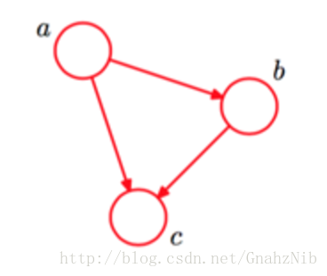
较复杂的贝叶斯网络,其对应的全概率公式为:
P(x1,x2,x3,x4,x5,x6,x7)=P(x1)P(x2)P(x3)P(x4∣x1,x2,x3)P(x5∣x1,x3)P(x6∣x4)P(x7∣x4,x5)<script type="math/tex; mode=display" id="MathJax-Element-251">P(x1, x2, x3, x4, x5, x6, x7)=P(x1)P(x2)P(x3)P(x4∣x1, x2, x3)P(x5∣x1, x3)P(x6∣x4)P(x7∣x4, x5)</script>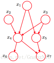
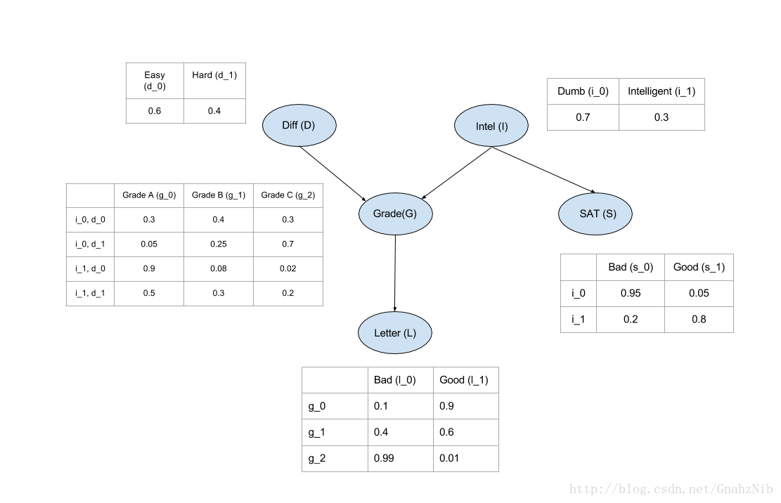
3、贝叶斯网络Student模型
一个学生拥有成绩、课程难度、智力、SAT得分、推荐信等变量。通过一张有向无环图可以把这些变量的关系表示出来,可以想象成绩由课程难度和智力决定,SAT成绩由智力决定,而推荐信由成绩决定。该模型对应的概率图如下:
4、通过概率图python类库pgmpy构建Student模型
代码如下:
from pgmpy.models import BayesianModel
from pgmpy.factors.discrete import TabularCPD

# 通过边来定义贝叶斯模型
model = BayesianModel([('D', 'G'), ('I', 'G'), ('G', 'L'), ('I', 'S')])

# 定义条件概率分布
cpd_d = TabularCPD(variable='D', variable_card=2, values=[[0.6, 0.4]])
cpd_i = TabularCPD(variable='I', variable_card=2, values=[[0.7, 0.3]])

# variable:变量
# variable_card:基数
# values:变量值
# evidence:
cpd_g = TabularCPD(variable='G', variable_card=3,
                   values=[[0.3, 0.05, 0.9,  0.5],
                           [0.4, 0.25, 0.08, 0.3],
                           [0.3, 0.7,  0.02, 0.2]],
                  evidence=['I', 'D'],
                  evidence_card=[2, 2])

cpd_l = TabularCPD(variable='L', variable_card=2,
                   values=[[0.1, 0.4, 0.99],
                           [0.9, 0.6, 0.01]],
                   evidence=['G'],
                   evidence_card=[3])

cpd_s = TabularCPD(variable='S', variable_card=2,
                   values=[[0.95, 0.2],
                           [0.05, 0.8]],
                   evidence=['I'],
                   evidence_card=[2])

# 将有向无环图与条件概率分布表关联
model.add_cpds(cpd_d, cpd_i, cpd_g, cpd_l, cpd_s)

# 验证模型:检查网络结构和CPD,并验证CPD是否正确定义和总和为1
model.check_model()
获取上述代码构建的概率图模型:
In[1]:model.get_cpds()
Out[1]:
[<TabularCPD representing P(D:2) at 0x10286e198>,
 <TabularCPD representing P(I:2) at 0x10286e160>,
 <TabularCPD representing P(G:3 | I:2, D:2) at 0x100d69710>,
 <TabularCPD representing P(L:2 | G:3) at 0x10286e1d0>,
 <TabularCPD representing P(S:2 | I:2) at 0x1093f6358>]
获取结点G的概率表:
In[2]:print(model.get_cpds('G'))
╒═════╤═════╤══════╤══════╤═════╕
│ I   │ I_0 │ I_0  │ I_1  │ I_1 │
├─────┼─────┼──────┼──────┼─────┤
│ D   │ D_0 │ D_1  │ D_0  │ D_1 │
├─────┼─────┼──────┼──────┼─────┤
│ G_0 │ 0.3 │ 0.05 │ 0.9  │ 0.5 │
├─────┼─────┼──────┼──────┼─────┤
│ G_1 │ 0.4 │ 0.25 │ 0.08 │ 0.3 │
├─────┼─────┼──────┼──────┼─────┤
│ G_2 │ 0.3 │ 0.7  │ 0.02 │ 0.2 │
╘═════╧═════╧══════╧══════╧═════╛
获取结点G的基数:
In[3]: model.get_cardinality('G')
Out[3]: 3
获取整个贝叶斯网络的局部依赖:
In[4]: model.local_independencies(['D', 'I', 'S', 'G', 'L'])
Out[4]:
(D _|_ I, S)
(I _|_ D)
(S _|_ D, L, G | I)
(G _|_ S | I, D)
(L _|_ I, S, D | G)
通过贝叶斯网络计算联合分布
条件概率公式如下:
Student模型中,全概率公式的表示:
通过本地依赖条件,可得:
由上面等式可得,联合分布产生于图中所有的CPD,因此编码图中的联合分布有助于减少我们所要存储的参数。
推导 Bayiesian Model
因此,我们可能想知道一个聪明的学生在艰难的课程中可能的成绩,因为他在SAT中打得很好。 因此,为了从联合分配计算这些值,我们必须减少给定的变量,即I=1<script type="math/tex" id="MathJax-Element-324"> I = 1 </script>,D=1<script type="math/tex" id="MathJax-Element-325"> D = 1 </script>,S=1<script type="math/tex" id="MathJax-Element-326"> S = 1 </script>,然后将L<script type="math/tex" id="MathJax-Element-327"> L </script>的其他变量边际化 得到
在知道一个聪明的学生、他的一门比较难的课程及其SAT成绩较高的情况。为了从联合分布计算这些值,必须减少给定的变量I=1<script type="math/tex" id="MathJax-Element-329"> I = 1 </script>,D=1<script type="math/tex" id="MathJax-Element-330"> D = 1 </script>,S=1<script type="math/tex" id="MathJax-Element-331"> S = 1 </script>,然后将L<script type="math/tex" id="MathJax-Element-332"> L </script>的其他变量边缘化得到
变量消除
如果我们只想计算G的概率,需要边缘化其他所给的参数
P(G)=∑D,I,L,SP(D,I,G,L,S)<script type="math/tex" id="MathJax-Element-376"> P(G) = \sum_{D, I, L, S} P(D, I, G, L, S) </script>
P(G)=∑D,I,L,SP(L|G)∗P(S|I)∗P(G|D,I)∗P(D)∗P(I)<script type="math/tex" id="MathJax-Element-377"> P(G) = \sum_{D, I, L, S} P(L|G) * P(S|I) * P(G|D, I) * P(D) * P(I) </script>
P(G)=∑D∑I∑L∑SP(L|G)∗P(S|I)∗P(G|D,I)∗P(D)∗P(I)<script type="math/tex" id="MathJax-Element-378"> P(G) = \sum_D \sum_I \sum_L \sum_S P(L|G) * P(S|I) * P(G|D, I) * P(D) * P(I) </script>
由于并非所有的条件分布都取决于所有的变量,我们可以推出内部的求和:
P(G)=∑D∑I∑L∑SP(L|G)∗P(S|I)∗P(G|D,I)∗P(D)∗P(I)<script type="math/tex" id="MathJax-Element-379"> P(G) = \sum_D \sum_I \sum_L \sum_S P(L|G) * P(S|I) * P(G|D, I) * P(D) * P(I) </script>
P(G)=∑DP(D)∑IP(G|D,I)∗P(I)∑SP(S|I)∑LP(L|G)<script type="math/tex" id="MathJax-Element-380"> P(G) = \sum_D P(D) \sum_I P(G|D, I) * P(I) \sum_S P(S|I) \sum_L P(L|G) </script>
In[5]:from pgmpy.inference import VariableElimination
infer = VariableElimination(model)
print(infer.query(['G']) ['G'])
╒═════╤══════════╕
│ G   │   phi(G) │
╞═════╪══════════╡
│ G_0 │   0.3620 │
├─────┼──────────┤
│ G_1 │   0.2884 │
├─────┼──────────┤
│ G_2 │   0.3496 │
╘═════╧══════════╛计算P(G|D=0,I=1)<script type="math/tex" id="MathJax-Element-399"> P(G | D=0, I=1) </script>的条件分布
P(G|D=0,I=1)=∑L∑SP(L|G)∗P(S|I=1)∗P(G|D=0,I=1)∗P(D=0)∗P(I=1)<script type="math/tex" id="MathJax-Element-400"> P(G | D=0, I=1) = \sum_L \sum_S P(L|G) * P(S| I=1) * P(G| D=0, I=1) * P(D=0) * P(I=1) </script>
P(G|D=0,I=1)=P(D=0)∗P(I=1)∗P(G|D=0,I=1)∗∑LP(L|G)∗∑SP(S|I=1)<script type="math/tex" id="MathJax-Element-401"> P(G | D=0, I=1) = P(D=0) * P(I=1) * P(G | D=0, I=1) * \sum_L P(L | G) * \sum_S P(S | I=1) </script>
在pgmpy中我们只需要省略额外参数即可计算出条件分布概率
In[6]: print(infer.query(['G'], evidence={'D': 0, 'I': 1}) ['G'])
╒═════╤══════════╕
│ G   │   phi(G) │
╞═════╪══════════╡
│ G_0 │   0.9000 │
├─────┼──────────┤
│ G_1 │   0.0800 │
├─────┼──────────┤
│ G_2 │   0.0200 │
╘═════╧══════════╛
新数据节点值的预测跟计算条件概率非常相似,我们需要查询预测变量的其他全部特征。困难在于通过分布概率去代替更多可能的变量状态。
In[7]: infer.map_query('G')
Out[7]: {'G': 2}
有“AI”的1024 = 2048,欢迎大家加入2048 AI社区
更多推荐

 20
20 0
0- 0


 已为社区贡献1条内容

所有评论(0)